Page 173 - Instrumentation Reference Book 3E

Methodsfor characterizing a group of particles 157
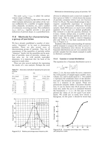
The ratio as/av = as,v is called the surface obvious is tabulation and a contrived example of
volume shape coefficient. this is given in Table 1 1.1 which shows the masses
The subject is covered by BS 4359 (1970) Pt I11 of particles contained within 5 pm size fractions
which includes definitions and tables of the vari- from 0 to 40 pm. The main disadvantage is that it
ous coefficients for a number of regular shapes: requires considerable experience to recognize
cubes, ellipsoids. tetrahedra, etc., and a number what could be important differences between
of commonly occurring particles. The coefficients samples. Such differences are much more readily
as,av and QS.V together provide a very good apparent if the results are plotted graphically.
indication of particle shape, in a quantified form. One method is to plot the quantity obtained. be
it mass, volume, surface area; or number of par-
ticles in each size fraction against size, both on a
11.6 Methods for characterizing linear scale. This is called a relative frequency
a group of particles plot and Table 11.1 has been transferred in this
way to Figure 11.2.
We have already established a number of alter- Students with a little understanding of statistics
native “diameters” to be used to characterize will be tempted to compare this with a normal or
particles. There are also several ways of Gaussian distribution (also shown). In practice,
characterizing groups of particles. They are all Gaussian distributions are not very common with
assessments of the quantities of particles within powder samples but this simple example is useful
“diameter” bands, but the quantities can be num- to illustrate a principle.
bers of particles. mass of particles, volume, sur-
face area, etc. As with particle equivalent
diameters, it is important that the basis of the 11.6.1 Gaussian or normal distributions
analysis is made clear. The equation for a Gaussian distribution curve is
There are also several methods for expressing
the results of a size analysis. Perhaps the most

Table 11.7 Alternative methods of tabulating the same size
analysis
(a) (b) where SJ’ dx, the area under the curve, represents
the total quantity of sample (again number, mass,
Size band 54 nzass Stated % less tlian volume, etc.) and is made equal to 1. The symbol
(P4 in band size stated size x represents the arithmetic mean of the distribu-
0-5 0.1 5 0.1 tion and CT the standard deviation of the distribu-
5-10 2.4 10 2.5 tion is a measure of the spread. These two
10-15 7.5 15 10.0 parameters uniquely define a Gaussian distribu-
15-20 50.0 20 60.0 tion. It can be shown that 68.26 percent of the
20-25 27.0 25 87.0 total area under the curve is contained between
25-30 12.5 30 99.5 the boundaries x = 2 f 0. In this case we have
>30 0.5 plotted the values of ySx for equal 5prn incre-
ments. We could just as easily have drawn a
histogram. At this point It should be stated that
60

50
d
40
E,
Lo
c
g 30
5
b
2 20
g
Q
10
0
5 5 10 15 20 25 30
Particle size (am)
Figure 11.3 Cumulative percentagemass-frequency
Figure 11.2 Relative percentage mass-frequency plot. plot using linear scales.