Page 174 - Instrumentation Reference Book 3E

158 Particle sizing

if any one of the distributions should turn out to The closeness of fit to a Gaussian distribution
be “normal” or Gaussian, then none of the other is much more obvious in Figure 11.4 than in
plots, i.e., number, volume, surface area distribu- Figures 11.2 and 11.3. With probability paper,
tions, will be Gaussian. small differences or errors at either extreme pro-
An advantage of the above presentation is that duce an exaggerated effect on the shape of the
small differences between samples would be read- line. This paper can still be used when the distri-
ily apparent. However, it would be useful to be bution is not “normal” but in this case, the line
able to measure easily the values of x and cr and will not be straight and standard deviation is no
this is not the case with the above. Two alterna- longer meaningful. If the distribution is not “nor-
tives are possible. One is to plot a cumulative mal” the 50 percent size is not the arithmetic
percentage frequency diagram, again on linear mean but is termed the median size. The arith-
axes, as in Figure 11.3. In this case one plots the metic mean needs to be calculated from
percentage less (or greater) than given sizes. 2 = C(percentage in size fraction
Alternatively, one can plot the same information x mean of size fraction)/lOO
on linear-probability paper where one axis, the
percentage frequency axis, is designed so that a and the basis on which it is calculated (mass,
Gaussian distribution will give a straight line, as surface, area, volume, or particle number) has to
in Figure 1 1.4. In a non-exact science such as size be stated. Each will give a different mean and
analysis, the latter has distinct advantages, but in median value.
either case the arithmetic mean X is the value of x
at the 50 percent point and the value of cr can 11.6.2 Log-normal distributions
be deduced as follows. Since 68.26 percent of a
normal distribution is contained between the It is unusual for powders to occur as Gaussian
values x = 2 + cr and x = 3 - cr, it follows that distributions. A plot as in Figure 11.2 would
typically be skewed towards the smaller particle
= Xg4% - 3 = 2 - sizes. Experience has shown, however, that pow-
1 der distributions often tend to be log-normal.
= 5 (X84% - x16%) Thus a percentage frequency plot with a logarith-
mic axis for the particle size reproduces a close
because x84%, - x16y0 covers the range of 68 per approximation to a symmetrical curve and a cumu-
cent of the total quantity. lative percentage plot on log-probability paper
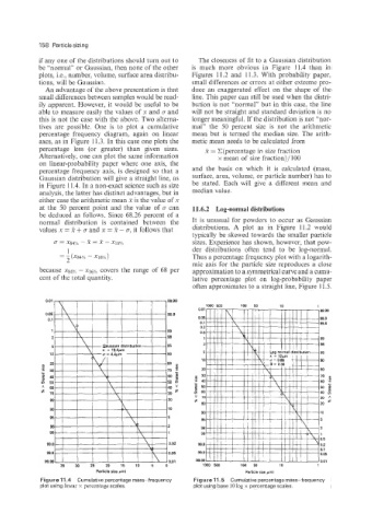
often approximates to a straight line, Figure 11.5.

1000 500 100 50 10
99 99
999
99 8
99
98
95
90
80
70 8
60 ,”
50
40 tj
30
20 *
10
5
2
1
05
02
01
0 05
0 01
1000 500 100 50 10 I
Particle size pml
Figure 11.4 Cumulative percentage mass-frequency Figure 11.5 Cumulative percentage mass-frequency
plot using linear x percentage scales. plot using base lolog x percentage scales