Page 536 - Instrumentation Reference Book 3E

Introduction 519

revealed by conducting a statistical analysis on a 21.1.1.1 Rndicsartive rieeccn,
series of repeated measurements. For errors in the
equipmenit or in the way it is operated the analysis Radioactive sousces have the property of disinte-
grating in a purely random manner, and the rate
uses the same source, and for source errors a of decay is given by the law
number of sources are used.
While statistical errors will follow a Gaussian
distribution, errors which are not random will not (22.8)
foilow such a distribution. so that if a series of
measurements cannot be fitted to a Gaussian dis- where X is called the decay constant and N is the
tribution curve then non-random errors must be total number of radioactive atoms present at zi
present. The chi-squared test allows one to test time t. This may be expressed as
the goodness of fit of a series of observations to N = iV0 exp (-At) (22.9)
the Gaussian distribution. If non-random errors
are not present, then the values of x' as deter- where No is the number of atoms of the parent
mined by the relation given in equation (22.7) substance present at some arbitrary time zero.
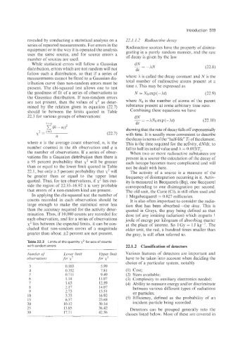
should lie between the limits quoted in Table Combining these equations we have
22.3 for various groups of observations: dN
- - --AN0 exp (-At) (22.10)
--
dt
showing that the rate of decay falls off exponentially
(22.7) with time. It is usually more convenient to describe
thedecay in terms ofthe "half-life" T+ oftheelement.
where ri is the average count observed. 11; is the This is the time required for the acfivity, dNldt, to
number counted in the ith observation and q is fall to half its initial value and X = O.693/Ti.
the nuniber of observations. If a series of obser- When two or more radioactive substahces are
vations fits a Gaussian distribution then there is present in a source the calculation of the decay of
a 95 percent probability that x2 will be greater each isotope becomes more complicated and will
than or equal to the lower limit quoted in Table not be dealt with here.
22.1, but only a 5 percent probability that y2 will The activity of a source is a measure of the
be greater than or equal to the upper limit frequency of disintegration occurring in it. Activ-
quoted. Thus, for ten observations, if x2 lies out- ity is measured in Becquerels (Bq), one
side the region of 22.33-16.92 it is very probable corresponding to one disintegration per second.
that errors of a non-random kind are present. The old unit, the Curie (Ci), is still often used and
In applying the chi-squared test the number of 1 Megabecquerel = 0.027 millicuries.
counts recorded in each observation should be It is also often important to consider the radia-
large enough to make the statistical error less tion that has been absorbed--the dose. This is
than the accuracy required for the activity deter- quoted in Grays, the gray being defined as that
mination. Thus, if 10,000 counts are recorded for dose (of any ionizing radiation) which imparts I
each observation, and for a series of observations joule of energy per kilogram of absorbing matter
y2 lies between the expected limits, it can be con- at the place of iiiterest. So 1 Gy = 9 J kg-l. The
cluded that non-random errors of a magnitude older unit, the rad, a hundred times smaller than
greater than about A2 percent are not present. the gray, is still often referred to.

Table 22.3 Limits of the quantity yz for sets of counts
with random errors 22.1.2 Classification of detectors
Number. of Lower limit L$pcr limit Various features of detectors are important and
observations for xz for h'2 have to be taken into account when deciding the
choice of a particular system, notably
3 0.103 5.99
4 0.352 7.81 (1) cost;
5 0.711 9.49 (2) Sizes available;
6 1.14 11.07 (3) Complexity in auxiliary electronics needed;
7 1.63 12.59 (4) Ability to measure energy and/or discriminate
8 2.17 14.07 between various different types of radiations
9 2.73 15.51 or particles;
10 3.33 16.92 (5) Efficiency, defined as the probability of ai1
15 6.57 23.68
20 10.12 30.14 incident particle being recorded.
25 13.85 36.41 Detectors can be grouped generally into the
30 17.71 42.56 classes listed below. Most of these are covered in