Page 29 - Integrated Wireless Propagation Models

I n t r o d u c t i o n t o M o d e l i n g M o bi l e S i g n a l s i n W i r e l e s s C o m m u n i c a t i o n s 7

t, Time
(a)

II)
"0
.£
&
c:
!!! r0(t)
..
iii
c:
C)
i:li
t, Time
(b)
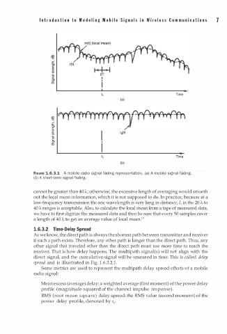
FIGURE 1.6.3.1 A mobile radio signal fading representation. (a) A mobile signal fadi n g.
(b) A short-term signal fading.

cannot be greater than 40 'A; otherwise, the excessive length of averaging would smooth
out the local mean information, which it is not supposed to do. In practice, because at a
L
low-frequency transmission the one wavelength is very long in distance, i n the 20 'A to
40 'A ranges is acceptable. Also, to calculate the local mean from a tape of measured data,
we have to first digitize the measured data and then be sure that every 50 samples cover
1
a length of 40 'A to get an average value of local mean. 9
1.6.3.2 Time-Delay Spread
As we know, the direct path is always the shortest path between transmitter and receiver
if such a path exists. Therefore, any other path is longer than the direct path. Thus, any
other signal that traveled other than the direct path must use more time to reach the
receiver. That is how delay happens. The multipath signal(s) will not align with the
direct signal, and the cumulative signal will be smeared in time. This is called delay
1
1
spread and is illustrated in Fig. . 6.3.2. .
o
Some metrics are used to represent the multipath delay spread effects f a mobile
radio signal:
Mean excess (average) delay: a weighted average (first moment) of the power delay
profile (magnitude squared of the channel impulse response).
s
RMS (root mean q u a r e ) delay spread: the RMS value (second moment) of the
p
power delay r ofile, denoted by sf