Page 42 - Intelligent Communication Systems

26 INTELLIGENT COMMUNICATION SYSTEMS
4.4 ASYNCHRONOUS TRANSFER MODE

Asynchronous transfer mode (ATM) provides high-speed switching functions. An
ATM packet is called an ATM cell of 53 octets, which consists of control infor-
mation and data. In a packet switching system, the packet size is variable. There-
fore it takes time to identify the packet size and process it. In an ATM switching
system, a packet size is 53 octets. Therefore it is easy to identify and process.
The network where switching systems, terminals, and transmission lines are
linked is called a network topology. Graph theory is used to solve problems con-
cerning network topology. A node corresponds to a switching system or a terminal.
A branch corresponds to a transmission line of a network. The transmission line has
characteristics such as transmission cost, distance, delay, capacity, and/or malfunc-
tion. The characteristics are evaluated and represented as the cost of a branch. The
problem of finding a path that has a minimum cost is called the "searching the short-
est path" problem. This problem can be solved by using a graph theory.
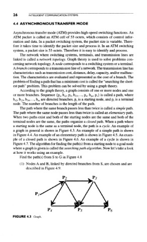
According to the graph theory, a graph consists of one or more nodes and one
or more branches. Sequence {p s , b s2, P 2, b23, • •, P n, b ns, P s} is called a path, where
b s2, b 23, b 34,..., b ns are directed branches, p s is a starting node, and p t, is a terminal
node. The number of branches is the length of the path.
The path where the same branch passes less than twice is called a simple path.
The path where the same node passes less than twice is called an elementary path.
When two paths exist and both of the starting nodes are the same and both of the
terminal nodes are the same, the paths organize a closed path. When a path where
a starting node is the same as a terminal node, the path is a cycle. An example of
a graph in general is shown in Figure 4.3. An example of a simple path is shown
in Figure 4.4. An example of an elementary path is shown in Figure 4.5. An exam-
ple of a closed path is shown in Figure 4.6. An example of a cycle is shown in
Figure 4.7. The algorithm for finding the path(s) from a starting node to a goal node
where a graph is given is called the searching path algorithm. Now let's take a look
at how it works using an example.
Find the path(s) from S to G in Figure 4.8

(1) Nodes A and B, linked by directed branches from S, are chosen and are
described in Figure 4.9.

FIGURE 4.3 Graph.