Page 153 - Intermediate Statistics for Dummies

12_045206 ch07.qxd 2/1/07 9:54 AM Page 132
132
Part II: Making Predictions by Using Regression
Bringing back polynomials
You may recall from algebra that a polynomial is a sum of x terms raised to a
variety of powers, and each x is preceded by a constant called the coefficient of
2
3
that term. For example, the model y = 2x + 3x + 6x is a polynomial. The general
3
k
2
1
form for a polynomial regression model is y = β 0 + β 1 x + β 2 x + β 3 x + . . . + β k x .
Here, k represents the total number of terms in the model.
2
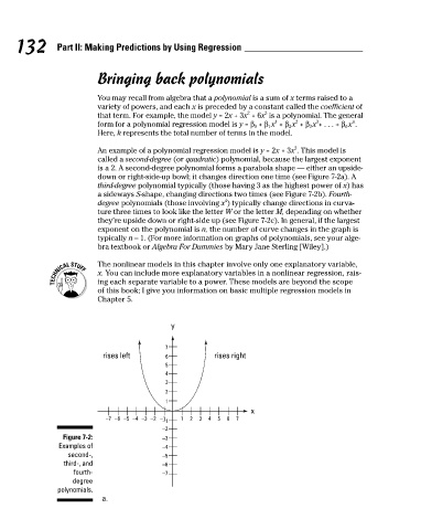
An example of a polynomial regression model is y = 2x + 3x . This model is
called a second-degree (or quadratic) polynomial, because the largest exponent
is a 2. A second-degree polynomial forms a parabola shape — either an upside-
down or right-side-up bowl; it changes direction one time (see Figure 7-2a). A
third-degree polynomial typically (those having 3 as the highest power of x) has
a sideways S-shape, changing directions two times (see Figure 7-2b). Fourth-
4
degree polynomials (those involving x ) typically change directions in curva-
ture three times to look like the letter W or the letter M, depending on whether
they’re upside down or right-side up (see Figure 7-2c). In general, if the largest
exponent on the polynomial is n, the number of curve changes in the graph is
typically n – 1. (For more information on graphs of polynomials, see your alge-
bra textbook or Algebra For Dummies by Mary Jane Sterling [Wiley].)
The nonlinear models in this chapter involve only one explanatory variable,
x. You can include more explanatory variables in a nonlinear regression, rais-
ing each separate variable to a power. These models are beyond the scope
of this book; I give you information on basic multiple regression models in
Chapter 5.
y
7
rises left 6 rises right
5
4
3
2
1
x
−7 −6 −5 −4 −3 −2 −1 1 2 3 4 5 6 7
−1
−2
Figure 7-2: −3
Examples of −4
second-, −5
third-, and −6
fourth- −7
degree
polynomials.
a.