Page 178 - Intermediate Statistics for Dummies

13_045206 ch08.qxd 2/1/07 10:02 AM Page 157
Chapter 8: Yes, No, Maybe So: Making Predictions by Using Logistic Regression
but here’s what’s happening: Chi-square goodness-of-fit tests measure the
overall difference between what you expect to see via your model versus
what you actually observe in your data. (Chapter 15 gives you the lowdown
on Chi-square tests.) The null hypothesis (Ho) for this test says you have a
difference of zero between what you observed and what you expected from
the model; that is, your model fits. The alternative hypothesis, denoted Ha,
says that the model doesn’t fit. If you get a small p-value (under 0.05), reject
Ho and conclude the model doesn’t fit. If you get a larger p-value (above 0.05),
you can stay with your model.
Failure to reject Ho here (having a large p-value) only means that you can’t
say your model doesn’t fit the population from which the sample came. It
doesn’t necessarily mean the model fits with 100 percent certainty. Your data
could be unrepresentative of the population just by chance.
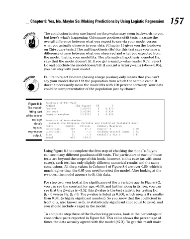
Goodness-of-Fit Test
Figure 8-4: The conclusion in step one based on the p-value may seem backwards to you, 157
Method Chi-Square DF P
The model- Pearson 2.83474 9 0.970
fitting part Deviance 3.63590 9 0.934
Hosmer-Lemeshow 2.75232 6 0.839
of the movie
and age Measures of Association:
data’s (Between the Response Variable and Predicted Probabilities)
Pairs Number Percent Summary Measures
logistic
Concordant 349 87.3 Somers’ D 0.80
regression Discordant 30 7.5 Goodman-Kruskal Gamma 0.84
output. Ties 21 5.3 Kendall’s Tau-a 0.41
Total 400 100.0
Using Figure 8-4 to complete the first step of checking the model’s fit, you
can see many different goodness-of-fit tests. The particulars of each of these
tests are beyond the scope of this book; however, in this case (as with most
cases), each test has only slightly different numerical results and the same
conclusions. All the p-values in Column 4 of Figure 8-4 are over 0.80, which is
much higher than the 0.05 you need to reject the model. After looking at the
p-values, the model appears to fit this data.
For step two, you look at the significance of the x variable age. In Figure 8-2,
you can see the constant for age, –0.18, and farther along in its row, you can
see that the Z-value is –3.52; this Z-value is the test statistic for testing Ho:
β 1 = 0 versus Ha: β 1 ≠ 0. The p-value is listed as 0.000, which means it’s smaller
than 0.001 (a highly significant number). So you know that the coefficient in
front of x, also known as β 1, is statistically significant (not equal to zero), and
you should include x (age) in the model.
To complete step three of the fit-checking process, look at the percentage of
concordant pairs reported in Figure 8-4. This value shows the percentage of
times the data actually agreed with the model (87.3). To get this result make