Page 176 - Intermediate Statistics for Dummies

13_045206 ch08.qxd 2/1/07 10:00 AM Page 155
Chapter 8: Yes, No, Maybe So: Making Predictions by Using Logistic Regression
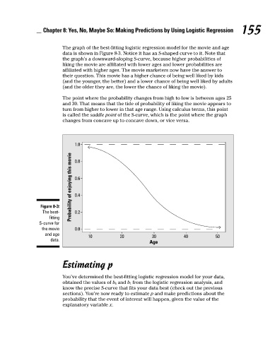
The graph of the best-fitting logistic regression model for the movie and age
data is shown in Figure 8-3. Notice it has an S-shaped curve to it. Note that
the graph’s a downward-sloping S-curve, because higher probabilities of
liking the movie are affiliated with lower ages and lower probabilities are
affiliated with higher ages. The movie marketers now have the answer to
their question. This movie has a higher chance of being well liked by kids
(and the younger, the better) and a lower chance of being well liked by adults
(and the older they are, the lower the chance of liking the movie).
The point where the probability changes from high to low is between ages 25
and 30. That means that the tide of probability of liking the movie appears to
turn from higher to lower in that age range. Using calculus terms, this point
is called the saddle point of the S-curve, which is the point where the graph
changes from concave up to concave down, or vice versa.
1.0 155
Probability of enjoying this movie 0.6
0.8
0.4
Figure 8-3:
The best- 0.2
fitting
S-curve for
the movie 0.0
and age
10 20 30 40 50
data.
Age
Estimating p

You’ve determined the best-fitting logistic regression model for your data,
obtained the values of b 0 and b 1 from the logistic regression analysis, and
know the precise S-curve that fits your data best (check out the previous
sections). You’re now ready to estimate p and make predictions about the
probability that the event of interest will happen, given the value of the
explanatory variable x.