Page 49 - Intermediate Statistics for Dummies

05_045206 ch01.qxd 2/1/07 9:41 AM Page 28
28
Part I: Data Analysis and Model-Building Basics
Finally, you may be interested in building a model for which a straight line
doesn’t fit. For example, you may want to predict miles per gallon, using the
speed of the car. While high speeds get low miles per gallon, low speeds can
get low miles per gallon as well. So the relationship between speed and miles
per gallon actually follows that of a parabola (an upside-down bowl, in this
case). This kind of relationship is called a quadratic relationship. More gener-
ally speaking, relationships that don’t follow a straight line are called nonlin-
ear relationships, and the technique you use to handle these situations is
called (no surprise) nonlinear regression. I get into the meat of this technique
in detail in Chapter 7.
Chi-square tests
Correlation and regression techniques all assume that the variable being
studied in most detail (the response variable) is quantitative. That is, the
variable measures or counts something. However, you can run into many sit-
uations where the data being studied isn’t quantitative, but rather qualitative.
In other words, the data themselves represent categories, not measurements
or counts.
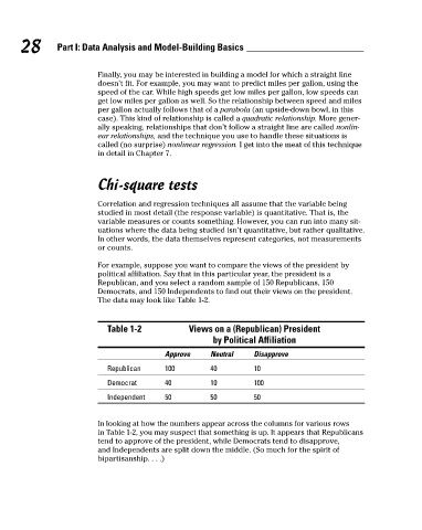
For example, suppose you want to compare the views of the president by
political affiliation. Say that in this particular year, the president is a
Republican, and you select a random sample of 150 Republicans, 150
Democrats, and 150 Independents to find out their views on the president.
The data may look like Table 1-2.
Table 1-2 Views on a (Republican) President
by Political Affiliation
Approve Neutral Disapprove
Republican 100 40 10
Democrat 40 10 100
Independent 50 50 50
In looking at how the numbers appear across the columns for various rows
in Table 1-2, you may suspect that something is up. It appears that Republicans
tend to approve of the president, while Democrats tend to disapprove,
and Independents are split down the middle. (So much for the spirit of
bipartisanship. . . .)