Page 231 - Intro to Tensor Calculus

225

◦
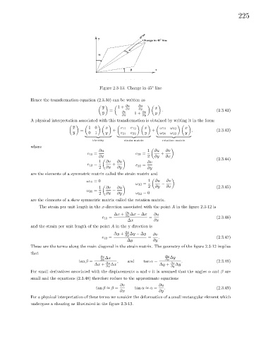
Figure 2.3-13. Change in 45 line

Hence the transformation equation (2.3.30) can be written as
∂u ∂u
x 1+ ∂x ∂y x
= . (2.3.42)
y ∂v 1+ ∂v y
∂x ∂y
A physical interpretation associated with this transformation is obtained by writing it in the form:

x 1 0 x e 11 e 12 x ω 11 ω 12 x
= + + , (2.3.43)
y 0 1 y e 21 e 22 y ω 21 ω 22 y
| {z } | {z } | {z }
identity strain matrix rotation matrix
where

∂u 1 ∂u ∂v
e 11 = e 21 = +
∂x 2 ∂y ∂x
(2.3.44)
1 ∂v ∂u ∂v
e 12 = + e 22 =
2 ∂x ∂y ∂y
are the elements of a symmetric matrix called the strain matrix and

ω 11 =0 1 ∂u ∂v
ω 12 = −

1 ∂v ∂u 2 ∂y ∂x (2.3.45)
ω 21 = −
2 ∂x ∂y ω 22 =0
are the elements of a skew symmetric matrix called the rotation matrix.
The strain per unit length in the x-direction associated with the point A in the figure 2.3-12 is
∆x + ∂u ∆x − ∆x ∂u
e 11 = ∂x = (2.3.46)
∆x ∂x
and the strain per unit length of the point A in the y direction is
∆y + ∂v ∆y − ∆y ∂v
∂y
e 22 = = . (2.3.47)
∆y ∂y
These are the terms along the main diagonal in the strain matrix. The geometry of the figure 2.3-12 implies
that
∂v ∆x ∂u ∆y
tan β = ∂x ∂u , and tan α = ∂y ∂v . (2.3.48)
∆x + ∆x ∆y + ∆y
∂x ∂y
For small derivatives associated with the displacements u and v it is assumed that the angles α and β are
small and the equations (2.3.48) therefore reduce to the approximate equations
∂v ∂u
tan β ≈ β = tan α ≈ α = . (2.3.49)
∂x ∂y
For a physical interpretation of these terms we consider the deformation of a small rectangular element which
undergoes a shearing as illustrated in the figure 2.3-13.