
Page 177 - INTRODUCTION TO THE CALCULUS OF VARIATIONS
P. 177
164 Isoperimetric inequality
Remark 6.17 (i) The proof that we will give is also valid in the case n =2.
However it is unduly complicated and less precise than the one given in the
preceding section.
(ii) Concerning the uniqueness that we will not prove below (cf. Berger [10],
Section 12.11), we should point out that it is a uniqueness only among convex
sets. In dimension 2, we did not need this restriction; since for a non convex set
A, its convex hull has larger area and smaller perimeter. In higher dimensions
this is not true anymore. In the case n ≥ 3, one can still obtain uniqueness by
assuming some regularity of the boundary ∂A, in order to avoid "hairy" spheres
(i.e., sets that have zero n and (n − 1) measures but non zero lower dimensional
measures).
n
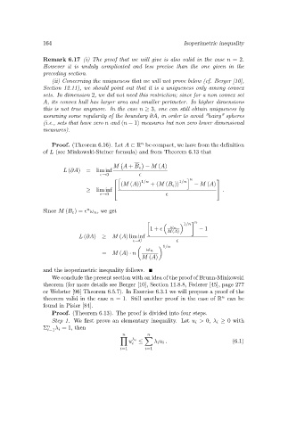
Proof. (Theorem 6.16). Let A ⊂ R be compact, we have from the definition
of L (see Minkowski-Steiner formula) and from Theorem 6.13 that
¡ ¢
M A + B − M (A)
L (∂A) = lim inf
→0
⎡ h 1/n 1/n i n ⎤
(M (A)) +(M (B )) − M (A)
≥ lim inf ⎣ ⎦ .
→0
n
Since M (B ε )= ω n ,weget
∙ ¸ n
³ ´ 1/n
1+ ω n − 1
M(A)
L (∂A) ≥ M (A) lim inf
→0
µ ¶ 1/n
ω n
= M (A) · n
M (A)
and the isoperimetric inequality follows.
We conclude the present section with an idea of the proof of Brunn-Minkowski
theorem (for more details see Berger [10], Section 11.8.8, Federer [45], page 277
or Webster [96] Theorem 6.5.7). In Exercise 6.3.1 we will propose a proof of the
n
theorem valid in the case n =1. Still another proof in the case of R can be
found in Pisier [84].
Proof. (Theorem 6.13). The proof is divided into four steps.
Step 1. We first prove an elementary inequality. Let u i > 0, λ i ≥ 0 with
i=1 i =1,then
Σ n λ
n n
Y X
u λ i ≤ λ i u i . (6.1)
i
i=1 i=1