Page 399 - Introduction to AI Robotics

382
11
mare computed for
)
In an occupancy grid, P (O js) and P (E Localization and Map Making y
js
ccupied
p
t
each element, g r[i][ i dthat is covered by a sensor scan. At each grid ele-
,
j
]
ment, the tuple of the two probabilities for that region is stored. A tuple can
be implemented as a C struct
typedef struct {
double occupied;
double empty;
}P;
P occupancy_grid[ROWS][COLUMNS];
Probabilities provide a representation for expressing the certainty about a
region g r[i][ i d There still needs to be a function which transfers a partic-
.
]
j
ular sonar reading into the probability for each grid element in a way that
captures Fig. 11.2. One set of functions which quantify this model into prob-
abilities is given below.
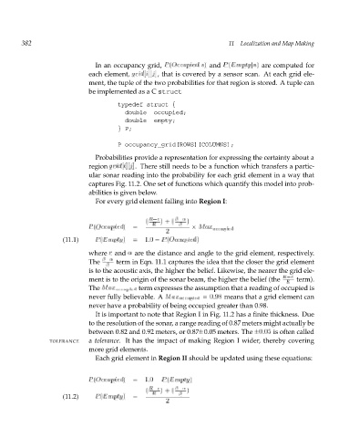
For every grid element falling into Region I:
( R R r ) ) + (
ccupied
P (O ) = M occupied a x
2
ccupied
(11.1) P (E ) m= 1:0 p P (O t y )
where r and are the distance and angle to the grid element, respectively.
The term in Eqn. 11.1 captures the idea that the closer the grid element

is to the acoustic axis, the higher the belief. Likewise, the nearer the grid ele-
ment is to the origin of the sonar beam, the higher the belief (the R r term).
R
a
The M occupied term expresses the xassumption that a reading of occupied is
never fully believable. A M occupied = :98 ameans that xa grid element can 0
never have a probability of being occupied greater than 0.98.
It is important to note that Region I in Fig. 11.2 has a finite thickness. Due
to the resolution of the sonar, a range reading of 0.87 meters might actually be
between 0.82 and 0.92 meters, or 0.87 0.05 meters. The 0:05 is often called
TOLERANCE a tolerance. It has the impact of making Region I wider, thereby covering
more grid elements.
Each grid element in Region II should be updated using these equations:

ccupied
mpty
P (O ) = 1:0 P (E )
( R R r ) ) + (
(11.2) P (E ) m= p t y
2