Page 400 - Introduction to AI Robotics

11.3 Bayesian
R=10 383
β=15

s=6

r=3.5
α=0

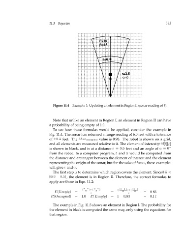
Figure 11.4 Example 1: Updating an element in Region II (sonar reading of 6).

Note that unlike an element in Region I, an element in Region II can have
a probability of being empty of 1.0.
To see how these formulas would be applied, consider the example in
Fig. 11.4. The sonar has returned a range reading of 6.0 feet with a tolerance
of 0:5 feet. The M occupied value a is 0.98. The xrobot is shown on a grid,
and all elements are measured relative to it. The element of interest g r[i][ i d
j
]
is shown in black, and is at a distance r = 3:5 feet and an angle of = 0
from the robot. In a computer program, r and would be computed from
the distance and arctangent between the element of interest and the element
representing the origin of the sonar, but for the sake of focus, these examples
will give r and .
The first step is to determine which region covers the element. Since 3:5 <
(6 :0 0:5) , the element is in Region II. Therefore, the correct formulas to
apply are those in Eqn. 11.2:

( R r )+( ) ( 10 3:5 )+( 15 0 )
P (E ) m= R p t y = 10 15 = 0:83
2 2
ccupied
mpty
P (O ) = 1:0 P (E ) = 1 0:83 = 0:17
The example in Fig. 11.5 shows an element in Region I. The probability for
the element in black is computed the same way, only using the equations for
that region.