Page 401 - Introduction to AI Robotics

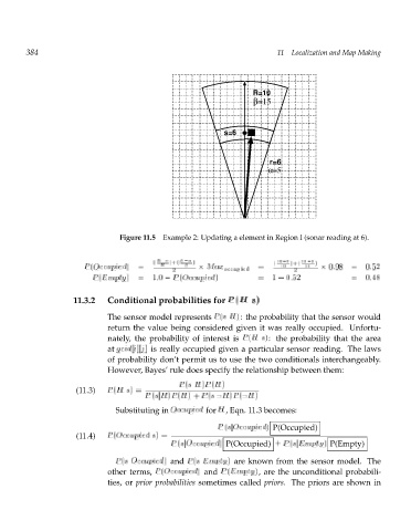
384
R=10 11 Localization and Map Making
β=15

s=6

r=6
α=5

Figure 11.5 Example 2: Updating a element in Region I (sonar reading at 6).

( R r )+( ) ( 10 6 )+( 15 5 )
P (O ) = R M occupied = a 10 15 x 0:98 = 0:52
ccupied
2 2
P (E ) m= 1:0 p P (O t y ) = 1 0:52 = 0:48
ccupied
11.3.2 Conditional probabilities for P (Hjs)
The sensor model represents P (sjH): the probability that the sensor would
return the value being considered given it was really occupied. Unfortu-
nately, the probability of interest is P (Hjs): the probability that the area
]
j
at g r[i][ i dis really occupied given a particular sensor reading. The laws
of probability don’t permit us to use the two conditionals interchangeably.
However, Bayes’ rule does specify the relationship between them:
P (sjH)P (H)
(11.3) P (Hjs) =
P (sjH)P (H) P (sj: H)P (: +H)
Substituting in O for H, Eqn. 11.3 becomes:
ccupied
ccupied
P (sjO ) P(Occupied)
ccupied
(11.4) P (O js) =
ccupied
P (sjO ) P(Occupied) + P (sjE ) mP(Empty) p t y
ccupied
P (sjO ) and P (sjE ) are known from the sensor model. The
mpty
other terms, P (Occupied ) and P (E ), are the unconditional probabili-
mpty
ties, or prior probabilities sometimes called priors. The priors are shown in