Page 238 - Introduction to Autonomous Mobile Robots

223
Mobile Robot Localization
each position. An example of just such a procedure is the sensory uncertainty field of
Latombe [141], in which the robot must find a trajectory that reaches its goal while maxi-
mizing its localization confidence on-line.

5.6.2.3 Case study 2: Markov localization using a grid map
The major weakness of a purely topological decomposition of the environment is the reso-
lution limitation imposed by such a granular representation. The position of the robot is
usually limited to the resolution of a single node in such cases, and this may be undesirable
for certain applications.
In this case study, we examine the work of Burgard and colleagues [49, 50] in which far
more precise navigation is made possible using a grid-based representation while still
employing the Markov localization technique.
The robot used by this research, Rhino, is an RWI B24 robot with twenty-four sonars
and two Sick laser rangefinders. Clearly, at the sensory level this robot accumulates greater
and more accurate range data than is possible with the handful of sonar sensors mounted on
Dervish. In order to make maximal use of these fine-grained sensory data, Rhino uses a 2D
geometric environmental representation of free and occupied space. This metric map is tes-
sellated regularly into a fixed decomposition grid with each cell occupying 4 to 64 cm in
various instantiations.
Like Dervish, Rhino uses multiple-hypothesis belief representation. In line with the far
improved resolution of the environmental representation, the belief state representation of
Rhino consists of a 15 × 15 × 15 3D array representing the probability of 15 3 possible
robot positions (see figure 5.23). The resolution of the array is 15 cm × 15 cm × 1° . Note
that unlike Dervish, which assumes its orientation is approximate and known, Rhino
explicitly represents fine-grained alternative orientations, and so its belief state formally
represents three degrees of freedom. As we have stated before, the resolution of the belief
state representation must match the environmental representation in order for the overall
system to function well.
Whereas Dervish made use of only perceptual events, ignoring encoder inputs and there-
fore metric distance altogether, Rhino uses the complete Markov probabilistic localization
approach summarized in section 5.6.2.1, including both an explicit action update phase and
a perception update phase at every cycle.
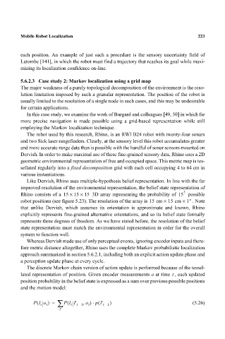
The discrete Markov chain version of action update is performed because of the tessel-
t
lated representation of position. Given encoder measurements o at time , each updated
position probability in the belief state is expressed as a sum over previous possible positions
and the motion model:

⋅
(
Pl o( ) = ∑ Pl l' o , ) pl' ) (5.26)
(
t t t t – 1 t t – 1
l'