Page 239 - Introduction to Autonomous Mobile Robots

224

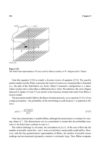
Figure 5.23 Chapter 5
The belief state representation 3D array used by Rhino (courtesy of W. Burgard and S. Thrun).

Note that equation (5.26) is simply a discrete version of equation (5.22). The specific
motion model used by Rhino represents the result of motion as a Gaussian that is bounded
(i.e., the tails of the distribution are finite). Rhino’s kinematic configuration is a three-
wheel synchro-drive rather than a differential-drive robot. Nevertheless, the error ellipses
depicted in figures 5.4 and 5.5 are similar to the Gaussian bounds that result from Rhino’s
motion model.
The perception model follows the Bayes formula precisely, as in equation (5.21). Given
i
l
a range perception the probability of the robot being at each location is updated as fol-
lows:
p il)p l()
(
(
p li) = ------------------------ (5.27)
pi()
Note that a denominator is used by Rhino, although the denominator is constant for vary-
l
ing values of . This denominator acts as a normalizer to ensure that the probability mea-
sures in the belief state continue to sum to 1.
The critical challenge is, of course, the calculation of p il( ) . In the case of Dervish, the
i
number of possible values for and were so small that a simple table could suffice. How-
l
ever, with the fine-grained metric representation of Rhino, the number of possible sensor
readings and environmental geometric contexts is extremely large. Thus, Rhino computes