Page 244 - Introduction to Autonomous Mobile Robots

229
Mobile Robot Localization
Static estimation. Suppose that our robot has two sensors, an ultrasonic range sensor and
a laser rangefinding sensor. The laser rangefinder provides far richer and more accurate
data for localization, but it will suffer from failure modes that differ from that of the sonar
ranger. For instance, a glass wall will be transparent to the laser but, when measured head-
on, the sonar will provide an accurate reading. Thus we wish to combine the information
provided by the two sensors, recognizing that such sensor fusion, when done in a principled
way, can only result in information gain.
The Kalman filter enables such fusion extremely efficiently, as long as we are willing to
approximate the error characteristics of these sensors with unimodal, zero-mean, Gaussian
noise. Specifically, assume we have taken two measurements, one with the sonar sensor at
time k and one with the laser rangefinder at time k + 1 . Based on each measurement indi-
vidually we can estimate the robot’s position. Such an estimate derived from the sonar is
q 1 and the estimate of position based on the laser is q 2 . As a simplified way of character-
izing the error associated with each of these estimates, we presume a (unimodal) Gaussian
probability density curve and thereby associate one variance with each measurement: σ 2 1
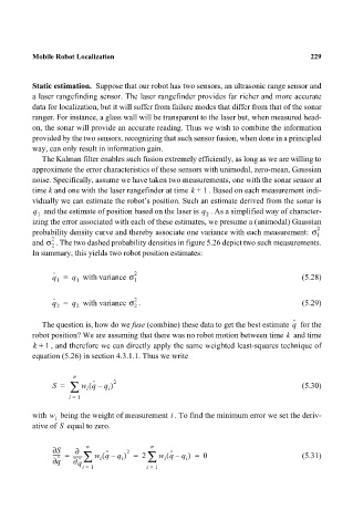
and σ 2 . The two dashed probability densities in figure 5.26 depict two such measurements.
2
In summary, this yields two robot position estimates:

ˆ
q = q 1 with variance σ 2 1 (5.28)
1
q ˆ = q 2 with variance σ 2 2 . (5.29)
2
q ˆ
The question is, how do we fuse (combine) these data to get the best estimate for the
robot position? We are assuming that there was no robot motion between time and time
k
k + 1 , and therefore we can directly apply the same weighted least-squares technique of
equation (5.26) in section 4.3.1.1. Thus we write

n
∑ w q ˆ –( q ) 2
S = i i (5.30)
i = 1

i
with w being the weight of measurement . To find the minimum error we set the deriv-
i
S
ative of equal to zero.
S ∂ ∂ n 2 n
(
----- = ∑ w q ˆ –( q ) = 2 ∑ w q ˆ – q ) = 0 (5.31)
q ˆ ∂ q ˆ ∂ i i i i
i = 1 i = 1