Page 245 - Introduction to Autonomous Mobile Robots

230

n n Chapter 5
∑ w q ˆ – ∑ w q = 0 (5.32)
i
i i
i = 1 i = 1
n
∑ w q
i i
-------------------
q ˆ = i = 1 (5.33)
n
∑ w i
i = 1

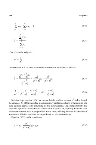
If we take as the weight w i

1
w = ----- (5.34)
i 2
σ
i
q ˆ
then the value of in terms of two measurements can be defined as follows:

1 1
-----q + -----q 2
1
σ 2 σ 2 σ 2 σ 2
1
2
2
1
q ˆ = ------------------------------ = ------------------q + ------------------q 2 (5.35)
1
1 1 2 2 2 2
----- + ----- σ + σ 2 σ + σ 2
1
1
σ 2 σ 2
1 2
2 σ 2 σ σ 2
2
1 1 1 σ + 1 2 1 2
2
----- = ----- + ----- = ------------------ ; σ = ------------------ 2 (5.36)
2
2
2
2 2
2
σ σ 1 σ 2 σ σ σ + σ 1
1 2
2
Note that from equation (5.36) we can see that the resulting variance σ 2 is less than all
the variances σ 2 of the individual measurements. Thus the uncertainty of the position esti-
i
mate has been decreased by combining the two measurements. The solid probability den-
sity curve represents the result of the Kalman filter in figure 5.26, depicting this result. Even
poor measurements, such as are provided by the sonar, will only increase the precision of
an estimate. This is a result that we expect based on information theory.
Equation (5.35) can be rewritten as
σ 2
1
q ˆ = q + ------------------ q –( 2 q ) (5.37)
1
1
2
2
σ + σ
1 2