Page 246 - Introduction to Autonomous Mobile Robots

Mobile Robot Localization

fq() 2 231
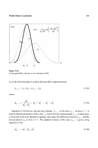
1  ( q – µ) 
fq() = -------------- exp –  ------------------- 
σ 2π  2σ 2 

q
q 2 q ˆ q 1

Figure 5.26
Fusing probability density of two estimates [106].

or, in the final form that is used in Kalman filter implementation,

x ˆ k + 1 = x ˆ + K k + 1 z ( k + 1 – x ˆ ) (5.38)
k
k
where

σ 2 k 2 2 2 2
K k + 1 = ------------------ 2 ; σ = σ 1 ; σ = σ 2 (5.39)
z
k
2
σ + σ z
k
Equation (5.38) tells us, that the best estimate x ˆ of the state x at time k + 1 is
k + 1 k + 1
equal to the best prediction of the value x ˆ k before the new measurement z k + 1 is taken, plus
a correction term of an optimal weighting value times the difference between z k + 1 and the
best prediction x ˆ at time k + 1 . The updated variance of the state x ˆ is given using
k k + 1
equation (5.36)
2
σ 2 = σ – K σ 2 (5.40)
k + 1 k k + 1 k