Page 248 - Introduction to Autonomous Mobile Robots

Mobile Robot Localization

fx() 2 233
–
1  ( x µ) 
fx() = --------------exp –  ------------------- 
σ 2π  2σ 2 
σ t()
k k

u

σ t( k + 1 )
k'

xt()
ˆ
ˆ
x t () x t ( k + 1 )
k
k
k'
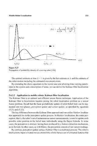
Figure 5.27
Propagation of probability density of a moving robot [106].
k
The optimal estimate at time k + 1 is given by the last estimate at and the estimate of
the robot motion including the estimated movement errors.
By extending the above equations to the vector case and allowing time-varying param-
eters in the system and a description of noise, we can derive the Kalman filter localization
algorithm.

5.6.3.2 Application to mobile robots: Kalman filter localization
The Kalman filter is an optimal and efficient sensor fusion technique. Application of the
Kalman filter to localization requires posing the robot localization problem as a sensor
fusion problem. Recall that the basic probabilistic update of robot belief state can be seg-
mented into two phases, perception update and action update, as specified by equations
(5.21) and (5.22).
The key difference between the Kalman filter approach and our earlier Markov localiza-
tion approach lies in the perception update process. In Markov localization, the entire per-
ception, that is, the robot’s set of instantaneous sensor measurements, is used to update each
possible robot position in the belief state individually using the Bayes formula. In some
cases, the perception is abstract, having been produced by a feature extraction mechanism,
as in Dervish. In other cases, as with Rhino, the perception consists of raw sensor readings.
By contrast, perception update using a Kalman filter is a multistep process. The robot’s
total sensory input is treated not as a monolithic whole but as a set of extracted features that