Page 253 - Introduction to Autonomous Mobile Robots

238

(
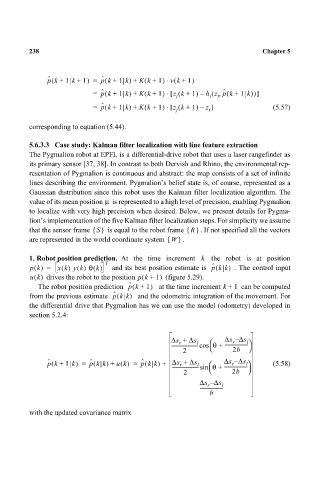
p k +( 1 k + 1) = p ˆ k + 1 k) + Kk + 1) vk + 1) Chapter 5
(
(
⋅
ˆ
(
p k +( 1 k + 1) = p ˆ k + 1 k) + Kk + 1) [⋅ z k +( 1) – h z p ˆ k + 1 k))]
(
(
(
ˆ
,
j i t
(
p k +( 1 k + 1) = p ˆ k + 1 k) + Kk + 1) [⋅ z k +( 1) – ] (5.57)
(
ˆ
z
j
t
corresponding to equation (5.44).
5.6.3.3 Case study: Kalman filter localization with line feature extraction
The Pygmalion robot at EPFL is a differential-drive robot that uses a laser rangefinder as
its primary sensor [37, 38]. In contrast to both Dervish and Rhino, the environmental rep-
resentation of Pygmalion is continuous and abstract: the map consists of a set of infinite
lines describing the environment. Pygmalion’s belief state is, of course, represented as a
Gaussian distribution since this robot uses the Kalman filter localization algorithm. The
µ
value of its mean position is represented to a high level of precision, enabling Pygmalion
to localize with very high precision when desired. Below, we present details for Pygma-
lion’s implementation of the five Kalman filter localization steps. For simplicity we assume
that the sensor frame S{} is equal to the robot frame R{} . If not specified all the vectors
are represented in the world coordinate system W{} .
1. Robot position prediction. At the time increment k the robot is at position
T
pk() = xk() yk() θ k() and its best position estimate is p ˆ kk( ) . The control input
u k() drives the robot to the position p k +( 1) (figure 5.29).
The robot position prediction p ˆ k +( 1) at the time increment k + 1 can be computed
from the previous estimate p ˆ kk( ) and the odometric integration of the movement. For
the differential drive that Pygmalion has we can use the model (odometry) developed in
section 5.2.4:

∆s + ∆s l  ∆s ∆– s l 
r
r
----------------------cos  θ + ------------------- 
2 2b
(
p k +( 1 k) = p ˆ kk) + uk() = p ˆ kk) + ∆s + ∆s l  ∆s ∆– s l  (5.58)
(
ˆ
r
r
----------------------sin  θ + ------------------- 
2 2b
∆s ∆– s l
r
-------------------
b
with the updated covariance matrix