Page 254 - Introduction to Autonomous Mobile Robots

Mobile Robot Localization

t=k+1 239
θ
(
pk + 1)

xk()
y pk() = yk()
t=k θ k()
x
{}
W

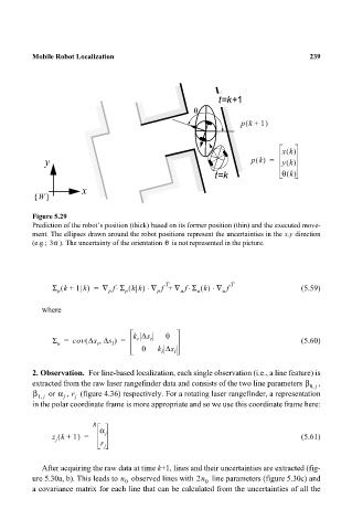
Figure 5.29
Prediction of the robot’s position (thick) based on its former position (thin) and the executed move-
ment. The ellipses drawn around the robot positions represent the uncertainties in the x,y direction
(e.g.; 3σ ). The uncertainty of the orientation is not represented in the picture.
θ

T
⋅
⋅
⋅
(
Σ k +( 1 k) = ∇ f Σ kk) ∇ f + ∇ f Σ k() ∇ f T (5.59)
⋅
p p p p u u u
where
(
,
r
Σ = cov ∆s ∆s ) = k ∆s r 0 (5.60)
l
u
r
0 k ∆s
l l
2. Observation. For line-based localization, each single observation (i.e., a line feature) is
extracted from the raw laser rangefinder data and consists of the two line parameters β 0 j ,
,
β or α , (figure 4.36) respectively. For a rotating laser rangefinder, a representation
r
,
1 j j j
in the polar coordinate frame is more appropriate and so we use this coordinate frame here:
R
α
(
z k + 1) = j (5.61)
j
r j
After acquiring the raw data at time k+1, lines and their uncertainties are extracted (fig-
ure 5.30a, b). This leads to n observed lines with 2n line parameters (figure 5.30c) and
0 0
a covariance matrix for each line that can be calculated from the uncertainties of all the