Page 251 - Introduction to Autonomous Mobile Robots

236

ˆ
ˆ
(
Z k +( 1) = { z k +( 1) 1 ≤≤ n )} Chapter 5
i
(5.49)
i
t
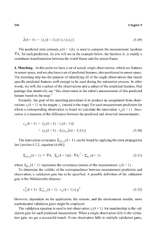
The predicted state estimate p ˆ k +( 1 k) is used to compute the measurement Jacobian
∇h i for each prediction. As you will see in the example below, the function h i is mainly a
coordinate transformation between the world frame and the sensor frame.
4. Matching. At this point we have a set of actual, single observations, which are features
in sensor space, and we also have a set of predicted features, also positioned in sensor space.
The matching step has the purpose of identifying all of the single observations that match
specific predicted features well enough to be used during the estimation process. In other
words, we will, for a subset of the observations and a subset of the predicted features, find
pairings that intuitively say “this observation is the robot’s measurement of this predicted
feature based on the map.”
Formally, the goal of the matching procedure is to produce an assignment from obser-
vations z k +( 1) to the targets (stored in the map). For each measurement prediction for
z
t
j
which a corresponding observation is found we calculate the innovation v k +( 1) . Inno-
ij
vation is a measure of the difference between the predicted and observed measurements:
(
(
v k +( 1) = [ z k + 1) – z ˆ k + 1)]
ij
i
j
(
(
,
v k +( 1) = [ z k + 1) – h z p ˆ k + 1 k))] (5.50)
(
i
j
ij
t
The innovation covariance Σ ( k + 1) can be found by applying the error propagation
,
IN ij
law [section 4.2.2, equation (4.60)]:
T
⋅
(
⋅
Σ IN ij ( k + 1) = ∇h Σ k + 1 k) ∇h + Σ Ri ( k + 1) (5.51)
,
,
i
i
p
where Σ ( k + 1) represents the covariance (noise) of the measurement z k +( 1) .
,
Ri i
To determine the validity of the correspondence between measurement prediction and
observation, a validation gate has to be specified. A possible definition of the validation
gate is the Mahalanobis distance:
T
1
v k +( 1) Σ – IN ij ( k + 1) v k + 1) ≤ g 2 (5.52)
⋅
⋅
(
,
ij
ij
However, dependent on the application, the sensors, and the environment models, more
sophisticated validation gates might be employed.
The validation equation is used to test observation z k +( 1) for membership in the val-
j
idation gate for each predicted measurement. When a single observation falls in the valida-
tion gate, we get a successful match. If one observation falls in multiple validation gates,