Page 267 - Introduction to Autonomous Mobile Robots

252

x Chapter 5
0
σ 2 σ y 0 r Updated
C = α αr Extracted line feature
αr
σ σ 2
αr r
{}
S
{} α
S
r
x
1
y Map feature
1
W
{} {} α α
W
r
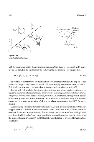
Figure 5.39
Uncertainties in the map.
with the covariance matrix Σ and an associated credibility factor between 0 and 1 quan-
c
t t
tifying the belief in the existence of the feature in the environment (see figure 5.39):
,
,
M = { z ˆ Σ c ( 1 ≤≤ n)} (5.69)
t
t t t
In contrast to the map used for Kalman filter localization previously, the map M is not
assumed to be precisely known because it will be created by an uncertain robot over time.
This is why the features are described with associated covariance matrices Σ .
z ˆ
t t
Just as with Kalman filter localization, the matching step yields has three outcomes in
regard to measurement predictions and observations: matched prediction and observations,
unexpected observations, and unobserved predictions. Localization, or the position update
of the robot, proceeds as before. However, the map is also updated now, using all three out-
comes and complete propagation of all the correlated uncertainties (see [23] for more
details).
An interesting variable is the credibility factor , which governs the likelihood that the
c
t
mapped feature is indeed in the environment. How should the robot’s failure to match
observed features to a particular map feature reduce that map feature’s credibility? And
also, how should the robot’s success at matching a mapped feature increase the chance that
the mapped feature is “correct?” In [23] the following function is proposed for calculating
credibility:

n n
 s u 
–  ----- – -----
b 
a
c k() = 1 – e (5.70)
t