Page 145 - Introduction to Computational Fluid Dynamics

P1: IWV
May 20, 2005
0 521 85326 5
12:28
0521853265c05
CB908/Date
124
WALL
SYMMETRY 2D CONVECTION – CARTESIAN GRIDS
c
d
e
f j = jn
WALL i = in Fin
EXIT
INFLOW b
c d e
i = 1
WALL
WALL Fin WALL
j = 1
a WALL b a WALL f
a) Exit Boundary b) Periodic Boundaries
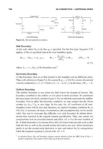
Figure 5.5. Exit and periodic boundaries.
Wall Boundary
At the wall, either b or its flux q b is specified. For the first type, Equation 5.76
applies. If flux is specified, then at the west boundary again,
A 1, j q 1, j
Su 2, j = Su 2, j + A 1, j q 1, j , 1, j = + 2, j , AW 2, j = 0,
AW 2, j
(5.77)
where A 1, j = r j x 2 j is the boundary area. 9

Symmetry Boundary
At this boundary, there is no flow normal to the boundary and no diffusion either.
Thus, with reference to Figure 5.4, for a scalar , q 1, j = 0.0. For vectors, the normal
velocity component u 1 (1, j)=0and u 2 (1, j) = u 2 (2, j). In all cases, AW 2, j = 0.

Outflow Boundary
The outflow boundary is one where the fluid leaves the domain of interest. The
boundary condition at the outflow or exit plane is most uncertain. To understand
the main issues involved, consider Figure 5.5(a) in which de represents the outflow
boundary. Now to affect the boundary condition, we may assume that the Peclet
number (u 1 x 1 /
)| b is very large. In this case, the AE coefficient of all near-
boundary nodes will be zero and, therefore, no explicit boundary condition b or
∂ /∂n| b is necessary. In many circumstances, this assumption may not be strictly
valid. One way to overcome this difficulty is to shift boundary de further down-
stream than required in the original domain specification. Thus, one carries out
computations over an extended domain and effect AE = 0 at the new location of
de. A third alternative is to assume that a fully developed state prevails at de so that
both the first as well as the second normal derivatives are zero. Most researchers
prefer to set the second-order derivative to zero and extract b by extrapolation
while the transport equation is solved with AE = 0.

9 In turbulent flows, the wall boundary requires special attention when the HRE form of the e–
model is employed. This matter will be taken up in the next section.