Page 149 - Introduction to Computational Fluid Dynamics

P1: IWV
May 20, 2005
12:28
CB908/Date
0521853265c05
128
J = JN 0 521 85326 5 2D CONVECTION – CARTESIAN GRIDS
INERT
REGION

X 2

X
INERT 1
REGION

J =1
I = 1 I = IN
DOMAIN TRUE APPROXIMATE
OF IRREGULAR BOUNDARY
INTEREST BOUNDARY
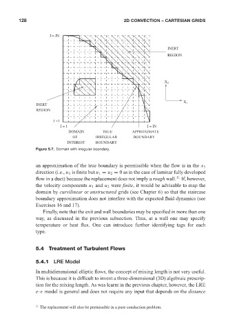
Figure 5.7. Domain with irregular boundary.

an approximation of the true boundary is permissible when the flow is in the x 3
direction (i.e., u 3 is finite but u 1 = u 2 = 0 as in the case of laminar fully developed
11
flow in a duct) because the replacement does not imply a rough wall. If, however,
the velocity components u 1 and u 2 were finite, it would be advisable to map the
domain by curvilinear or unstructured grids (see Chapter 6) so that the staircase
boundary approximation does not interfere with the expected fluid dynamics (see
Exercises 16 and 17).
Finally, note that the exit and wall boundaries may be specified in more than one
way, as discussed in the previous subsection. Thus, at a wall one may specify
temperature or heat flux. One can introduce further identifying tags for each
type.

5.4 Treatment of Turbulent Flows

5.4.1 LRE Model

In multidimensional elliptic flows, the concept of mixing length is not very useful.
This is because it is difficult to invent a three-dimensional (3D) algebraic prescrip-
tion for the mixing length. As was learnt in the previous chapter, however, the LRE
e– model is general and does not require any input that depends on the distance

11 The replacement will also be permissible in a pure conduction problem.