Page 147 - Introduction to Computational Fluid Dynamics

P. 147

P1: IWV
12:28
May 20, 2005
CB908/Date
0521853265c05
126
m 0 521 85326 5 e 2D CONVECTION – CARTESIAN GRIDS
d
n
JN
12
11
10
9
8 c f g
b
7
6
5 h
4 i
3
2
a l
j
2 3 4 56 7 8 910 11 12 13 14 15 16 IN
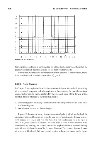
Figure 5.6. Node tagging.

the boundary condition is implemented by setting the boundary coefﬁcient of the
pressure-correction equation to zero for the near-boundary node.
Sometimes, we may have a boundary on which pressure is speciﬁed and, there-
fore, remains ﬁxed. For such boundaries, p = 0.
m,b

5.3.6 Node Tagging
In Chapter 2, we emphasised that the introduction of Su and Sp can facilitate writing
of generalised computer codes by capturing a large variety. In multidimensional
codes, further variety can be captured by tagging each node of the domain with a
number. This is intended to facilitate handling of

1. different types of boundary conditions over different portions of the same phys-
ical boundary and
2. domains that are not perfect rectangles.

Figure 5.6 shows an arbitrary domain a-b-c-d-e-f-g-h-i-j, which we shall call the
domain of interest. However, we regard it as a part of a rectangular domain a-m-n-l
with nodes i = 1to IN and j = 1to JN. This will create areas b-c-d-m, f-g-n-e,
and j-l-h-i, which are not of interest. We term them as inert or blocked areas. Now,
coordinates x 1i and x 2 j are chosen so that the implied cell-face locations exactly
coincide with the boundaries of the domain of interest. This ensures that our domain
of interest is ﬁlled with full (not partial) control volumes as shown in the ﬁgure.

142 143 144 145 146 147 148 149 150 151 152