Page 151 - Introduction to Computational Fluid Dynamics

P1: IWV
CB908/Date
0 521 85326 5
0521853265c05
130
2D CONVECTION – CARTESIAN GRIDS
13
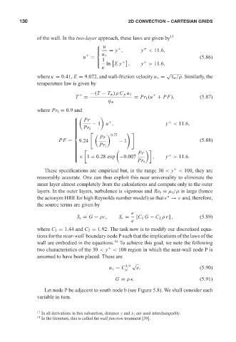
of the wall. In the two-layer approach, these laws are given by May 20, 2005 12:28
⎧ u
+
= y , y < 11.6,
+
⎪
⎨
u τ
+
u = (5.86)
⎪ 1
+
⎩ ln Ey + , y > 11.6,
κ
√
where κ = 0.41, E = 9.072, and wall-friction velocity u τ = τ w /ρ. Similarly, the
temperature law is given by
−(T − T w )ρ C p u τ
T + = = Pr t (u + PF), (5.87)
+
q w
where Pr t = 0.9 and
⎧
Pr
− 1 u , y < 11.6,
⎪ + +
⎪
⎪
Pr t
⎪
⎪
⎪
⎪

⎪
0.75
Pr
⎨
PF = 9.24 − 1 (5.88)
Pr t
⎪
⎪
⎪
⎪
Pr

⎪
⎪
+
⎩× 1 + 0.28 exp −0.007 , y > 11.6.
⎪
⎪
Pr t
These specifications are empirical but, in the range 30 < y < 100, they are
+
reasonably accurate. One can thus exploit this near universality to eliminate the
inner layer almost completely from the calculations and compute only in the outer
layers. In the outer layers, turbulence is vigorous and Re t = µ t /µ is large (hence
the acronym HRE for high Reynolds number model) so that → and, therefore,
∗
the source terms are given by

S e = G − ρ , S = [C 1 G − C 2 ρ ] , (5.89)
e
where C 1 = 1.44 and C 2 = 1.92. The task now is to modify our discretised equa-
tions for the near-wall boundary node P such that the implications of the laws of the
wall are embodied in the equations. 14 To achieve this goal, we note the following
two characteristics of the 30 < y < 100 region in which the near-wall node P is
+
assumed to have been placed. These are
√
u τ = C 1/4 e, (5.90)
µ
G = ρ . (5.91)
Let node P be adjacent to south node b (see Figure 5.8). We shall consider each
variable in turn.
13 In all derivations in this subsection, distance y and x 2 are used interchangeably.
14 In the literature, this is called the wall function treatment [39].