Page 150 - Introduction to Computational Fluid Dynamics

P1: IWV
CB908/Date
May 20, 2005
0 521 85326 5
0521853265c05
5.4 TREATMENT OF TURBULENT FLOWS
fromthewall.The2DellipticversionofthismodelcanbedescribedviaEquation5.1 12:28 129
∗
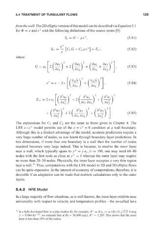
for = e and with the following definitions of the source terms [9]:
∗
S e = G − ρ , (5.81)
∗

S = C 1 G − C 2 ρ ∗ + E , (5.82)
∗
∗
e
where

2 2 2
∂u 1 ∂u 2 ∂u 2 ∂u 1
G = µ t 2 + 2 + + , (5.83)
∂x 1 ∂x 2 ∂x 1 ∂x 2
√ 2 √ 2

∂ e ∂ e
∗
= − 2ν + , (5.84)
∂x 1 ∂x 2
2 2 2
2 2 2

∂ u 1 ∂ u 1 ∂ u 1
E = 2νν t 2 + 2 + 2
∗
∂x 1 ∂x 1 ∂x 2 ∂x 2
2 2 2
2 2 2
∂ u 2 ∂ u 2 ∂ u 2
+ 2 + 2 + 2 . (5.85)
∂x 1 ∂x 1 ∂x 2 ∂x 2
The expressions for C 1 and C 2 are the same as those given in Chapter 4. The
∗
LRE e− model permits use of the e = = 0 condition at a wall boundary.
∗
Although this is a distinct advantage of the model, accurate predictions require a
very large number of nodes, as was learnt through boundary layer predictions. In
two dimensions, if more than one boundary is a wall then the number of nodes
required becomes very large indeed. This is because, to resolve the inner layer
near a wall, which typically spans to y = yu τ /ν = 100, one may need 60–80
+
nodes with the first node as close as y = 1 whereas the outer layer may require
+
no more than 20–30 nodes. Physically, the inner layer occupies a very thin region
12
near a wall. Thus, computations with the LRE model in 2D and 3D elliptic flows
can be quite expensive. In the interest of economy of computations, therefore, it is
desirable if an adaptation can be made that restricts calculations only to the outer
layers.

5.4.2 HRE Model

In a large majority of flow situations, as is well known, the inner layer exhibits near
universality with respect to velocity and temperature profiles – the so-called laws

√
12 In a fully developed flow in a pipe (radius R), for example, R = Ru τ /ν = (Re/2) f/2. Using
+
+
f = 0.046 Re −0.2 , we estimate that at Re = 50,000 (say), R = 1,285. This shows that the inner
layer is less than 10% of the radius.