Page 152 - Introduction to Computational Fluid Dynamics

P1: IWV
0 521 85326 5
CB908/Date
0521853265c05
5.4 TREATMENT OF TURBULENT FLOWS

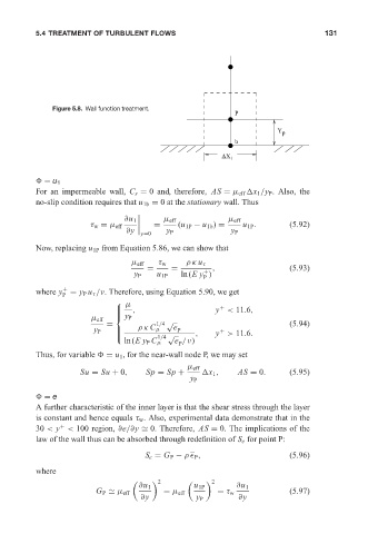
Figure 5.8. Wall function treatment. May 20, 2005 12:28 131
P
Y p
b

∆X 1

= u 1
For an impermeable wall, C s = 0 and, therefore, AS = µ eff x 1 /y P . Also, the
no-slip condition requires that u 1b = 0atthe stationary wall. Thus

∂u 1 µ eff µ eff
τ w = µ eff = (u 1P − u 1b ) = u 1P . (5.92)
∂y y P y P
y=0
Now, replacing u 1P from Equation 5.86, we can show that

µ eff τ w ρκ u τ
= = , (5.93)
+
y P u 1P ln(Ey )
P
+
where y = y P u τ /ν. Therefore, using Equation 5.90, we get
P
⎧ µ
, y < 11.6,
+
⎪
⎪
⎨ y P
µ eff
= 1/4 √ (5.94)
ρκ C µ e
y P ⎪ P +
⎪ √ , y > 11.6.
1/4
⎩
ln(Ey P C µ e /ν)
P
Thus, for variable = u 1 , for the near-wall node P, we may set
µ eff
Su = Su + 0, Sp = Sp + x 1 , AS = 0. (5.95)
y P
= e
A further characteristic of the inner layer is that the shear stress through the layer
is constant and hence equals τ w . Also, experimental data demonstrate that in the
30 < y < 100 region, ∂e/∂y
0. Therefore, AS = 0. The implications of the
+
law of the wall thus can be absorbed through redefinition of S e for point P:
S e = G P − ρ P , (5.96)
where
2 2
∂u 1 u 1P ∂u 1
G P
µ eff = µ eff = τ w (5.97)
∂y y P ∂y