Page 239 - Introduction to Computational Fluid Dynamics

P1: IBE
CB908/Date
0 521 85326 5
0521853265c07
218
PHASE CHANGE
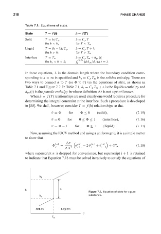
Table 7.1: Equations of state. May 25, 2005 11:14
State T = f(h) h = f(T)
Solid T = h/C p h = C p T
for h < h s for T < T m
Liquid T = (h − λ)/C p h = C p T + λ
for h > h l for T > T m
Interface T = T m h = C p T m + h ps (t)
t+ t

for h s < h < h l (dh ps /dt) dt = λ
t
In these equations, L is the domain length where the boundary condition corre-
sponding to x =∞ is specified and h s = C p T m is the solidus enthalpy. There are
two ways to connect h to T (or to θ) via the equations of state, as shown in
Table 7.1 and Figure 7.2. In Table 7.1, h l = C p T m + λ is the liquidus enthalpy and
h ps (t)isthe psuedo-enthalpy in whose definition t is not a priori known.
Whenh = f (T )relationshipsareused,clearlyonewouldrequireaprocedurefor
determining the integral constraint at the interface. Such a procedure is developed
in [85]. We shall, however, consider T = f (h) relationships so that

θ = for ≤ 0 (solid), (7.15)
θ = 0 for 0 ≤ ≤ 1 (interface), (7.16)

θ = − 1 for ≥ 1 (liquid). (7.17)
Now, assuming the IOCV method and using a uniform grid, it is a simple matter
to show that
τ l+1 l+1 l+1 o
l+1
= θ − 2θ + θ + , (7.18)
j 2 j+1 j j−1 j
X
where superscript n is dropped for convenience, but superscript l + 1 is retained
to indicate that Equation 7.18 must be solved iteratively to satisfy the equations of

h l

λ
h
Figure 7.2. Equation of state for a pure
h s substance.

SOLID LIQUID
T
T m