Page 241 - Introduction to Computational Fluid Dynamics

P1: IBE
CB908/Date
0521853265c07
220
PHASE CHANGE
2.0 0 521 85326 5 May 25, 2005 11:14
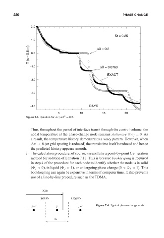
St = 0.25
1.0
T (x = 0.5 m) 0.0 ∆X = 0.2

−1.0 ∆X = 0.0769

EXACT
−2.0

−3.0

−4.0 DAYS
5 10 15 20
2
Figure 7.3. Solution for τ/ X = 0.2.

Thus, throughout the period of interface transit through the control volume, the
nodal temperature at the phase-change node remains stationary at θ j = 0. As
a result, the temperature history demonstrates a wavy pattern. However, when
x → 0 (or grid spacing is reduced) the transit time itself is reduced and hence
the predicted history appears smooth.
3. The calculation procedure, of course, necessitates a point-by-point GS iteration
method for solution of Equation 7.18. This is because bookkeeping is required
in step 4 of the procedure for each node to identify whether the node is in solid
( j < 0), in liquid ( j > 1), or undergoing phase change (0 < j < 1). This
bookkeeping can again be expensive in terms of computer time. It also prevents
use of a line-by-line procedure such as the TDMA.

(t)
X i
SOLID LIQUID

j − 1 j j + 1 Figure 7.4. Typical phase-change node.

∆x