Page 237 - Introduction to Computational Fluid Dynamics

P1: IBE
CB908/Date
0 521 85326 5
0521853265c07
216
PHASE CHANGE
T sup May 25, 2005 11:14
T l
SOLID LIQUID
T m
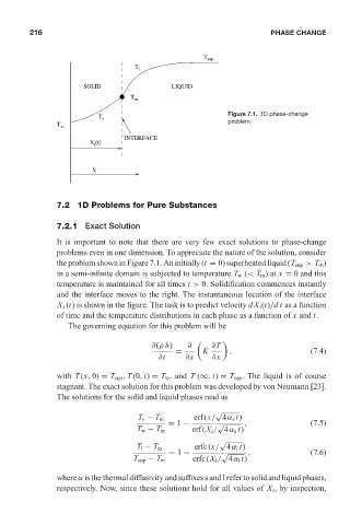
T s Figure 7.1. 1D phase-change
T w problem.
INTERFACE
X (t)
i

X

7.2 1D Problems for Pure Substances

7.2.1 Exact Solution

It is important to note that there are very few exact solutions to phase-change
problems even in one dimension. To appreciate the nature of the solution, consider
the problem shown in Figure 7.1. An initially (t = 0) superheated liquid (T sup > T m )
in a semi-infinite domain is subjected to temperature T w (< T m )at x = 0 and this
temperature is maintained for all times t > 0. Solidification commences instantly
and the interface moves to the right. The instantaneous location of the interface
X i (t) is shown in the figure. The task is to predict velocity dX i (t)/dt as a function
of time and the temperature distributions in each phase as a function of x and t.
The governing equation for this problem will be

∂(ρ h) ∂ ∂T
= K , (7.4)
∂t ∂x ∂x

with T (x, 0) = T sup , T (0, t) = T w , and T (∞, t) = T sup . The liquid is of course
stagnant. The exact solution for this problem was developed by von Neumann [23].
The solutions for the solid and liquid phases read as
√
erf(x/ 4α s t)
T s − T m
= 1 − √ , (7.5)
T w − T m erf(X i / 4α s t)
√
erfc(x/ 4α l t)
T l − T m
= 1 − √ , (7.6)
T sup − T m erfc(X i / 4α l t)
where α is the thermal diffusivity and suffixes s and l refer to solid and liquid phases,
respectively. Now, since these solutions hold for all values of X i , by inspection,