Page 232 - Introduction to Computational Fluid Dynamics

P1: IWV
CB908/Date
0 521 85326 5
0521853265c06
EXERCISES
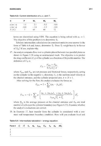
Table 6.3: Current distribution of u, v, and T. May 25, 2005 11:10 211
Φ P M 1 M 2 M 3
u (m / s) 1.1 2.1 −0.3 −0.8
v (m/s) −0.8 −1.0 −1.5 −0.8
◦
T ( C) ? 65 80 72

terms are discretised using UDS. The equation is being solved with α T = 1.
The objective of this problem is to determine T P .
Tabulate intermediate calculations (in consistent units) to your answer in the
form of Table 6.4 and, hence, determine T P . Does T P weigh heavily in favour
? If yes, explain why.
of T M 2
17. An analyst computes flow over a cylinder placed between two parallel plates as
shown in Figure 5.28 using an unstructured mesh. The objective is to predict
the drag coefficient (C D ) of the cylinder as a function of Reynolds number. The
definition of C D is

F pres + F fric
C D = ,
2
0.5ρ U A
o
where F pres and F fric are net pressure and frictional forces, respectively, acting
on the cylinder in the negative x 1 direction, U o is the uniform axial velocity at
the channel entrance, and the cylinder projected area A = D × 1.
After solving for the flow, the analyst evaluates the forces as
1
F pres = 2 × (p B − p )β ,
in 1
K B
⎡ ⎤

(u 1 + u 1 ) P l x 1 + (u 2 + u 2 ) P l x 2 1
F fric =−2 × µ ⎣ % ⎦ β ,
1
2
l + l 2
K B l P 2 B
x 1 x 2
where p in is the average pressure at the channel entrance and K B are total
number of cells near the cylinder boundary (see Figure 6.33). Examine whether
the analyst’s evaluations are correct.
18. In Exercise 17, heat transfer from the cylinder is considered with a con-
stant wall temperature boundary condition. How will you evaluate local and

Table 6.4: Intermediate tabulation – energy equation.

Face k β 1 β 2
1 1 f m A fk l P 2 E 2 C ck f ck d ck AE k
1
2
3