Page 231 - Introduction to Computational Fluid Dynamics

P1: IWV
May 25, 2005
11:10
CB908/Date
0521853265c06
210
1
6 0 521 85326 5 5 2D CONVECTION – COMPLEX DOMAINS
M 2 M 1
P
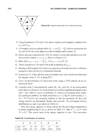
3 2 Figure 6.32. Neighbouring cells of an unstructured mesh.
M 3
4

8. Using Equations 6.125 and 6.126, derive explicit exit boundary conditions for
u 1,B and u 2,B .
4
4
9. A boundary receives radiant influx F B = σ(T − T ). Derive expressions for
∞ B
Su and Sp for the node adjacent to this boundary and evaluate T B .
u
10. Derive an exact expression for AP by control-volume discretisation over cell-
ck
face control volume c 1 –c 2 –c 3 –c 4 shown in Figure 6.13.
2 i 2 2
=| β (x i,E − x i,P )|β /A .
i=1 1 1 c
11. Show that x 2,E 2 − x 2,P 2
12. Verify Equations 6.139 and 6.140 in the evaluation of p x 2 ,P .
13. Starting with Equation 6.62, derive an expression for total convective–diffusive
transport at the cell face of a tetrahedral element.
14. In Exercise 13, if the cell face were a boundary face, how would you determine
the tangent vector t 2 if t 1 is along PP 2 ?
15. Carry out discretisation of convection terms using a TVD scheme on an un-
structured mesh.
16. Consider node P surrounded by nodes M 1 ,M 2 , and M 3 of an unstructured
mesh shown in Figure 6.32. Each element is a perfect equilateral triangle (each
side 1 cm). Table 6.2 gives coordinates of vertices surrounding these nodes.
3
In a particular problem, the fluid properties (ρ = 1.2 kg/m and viscosity µ =
−6
2
15 × 10 N-s/m ) are assumed constant so that the equations for flow and
energy transfer are decoupled. Steady state prevails. The converged velocity
distributions (u and v) are shown in Table 6.3.
Now, the energy equation is being solved and the prevailing temperatures
T
at nodes neighbouring P are as shown in Table 6.3. Take
= µ/Pr with
Pr = 0.7. The source term in the energy equation is zero. The convection

Table 6.2: Coordinates of vertices.

1 2 3 4 5 6
x (cm) 0.5 1.0 0.0 0.5 1.5 −0.5
y (cm) 0.866 0.0 0.0 −0.866 0.866 0.866