Page 228 - Introduction to Computational Fluid Dynamics

P1: IWV
May 25, 2005
CB908/Date
0521853265c06
0 521 85326 5
6.5 CLOSURE

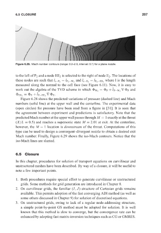
Figure 6.29. Mach number contours (range: 0.2–2.0, interval: 0.1) for a plane nozzle. 11:10 207

to the left of P 2 and a node EE 2 is selected to the right of node E 2 . The locations of
where l is the length
these nodes are such that l c−P 2 = l P 2 −W 2 and l c−E 2 = l E 2 −EE 2
measured along the normal to the cell face (see Figure 6.11). Now, it is easy to
∇ P and
work out the algebra of the TVD scheme in which W 2 = P + l P−W 2
∇ E .
EE 2 = E + l E−EE 2
Figure 6.28 shows the predicted variations of pressure (dashed line) and Mach
numbers (solid line) at the upper wall and the centerline. The experimental data
(open circles) for pressure have been read from a figure in [31]. It is seen that
the agreement between experiment and predictions is satisfactory. Note that the
predicted Mach number at the upper wall passes through M = 1 exactly at the throat
(X/L = 0.5) and reaches a supersonic state M = 2.01 at exit. At the centerline,
however, the M = 1 location is downstream of the throat. Computations of this
type can be used to design a convergent–divergent nozzle to obtain a desired exit
Mach number. Finally, Figure 6.29 shows the iso-Mach contours. Notice that the
iso-Mach lines are slanted.

6.5 Closure
In this chapter, procedures for solution of transport equations on curvilinear and
unstructured meshes have been described. By way of a closure, it will be useful to
note a few important points.

1. Both procedures require special effort to generate curvilinear or unstructured
grids. Some methods for grid generation are introduced in Chapter 8.
2. On curvilinear grids, the familiar (I, J) structure of Cartesian grids remains
available. This permits adoption of the fast converging ADI method (as well as
some others discussed in Chapter 9) for solution of discretised equations.
3. On unstructured grids, owing to lack of a regular node-addressing structure,
a simple point-by-point GS method must be adopted for solution. It is well
known that this method is slow to converge, but the convergence rate can be
enhanced by adopting fast matrix-inversion techniques such as CG or GMRES.