Page 224 - Introduction to Computational Fluid Dynamics

P1: IWV
CB908/Date
0 521 85326 5
0521853265c06
6.4 APPLICATIONS

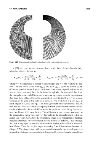
Figure 6.23. Unstructured meshes for natural convection in an eccentric annulus. May 25, 2005 11:10 203

In [37], the experimental data are plotted in the form of a local conductivity
ratio K eq , which is defined as

q w,i (θ)R i R o q w,o (θ)R o R o
K eq,i (θ) = ln , K eq,o (θ) = ln , (6.145)
K (T h − T c ) R i K (T h − T c ) R i
where θ = 0 corresponds to the top of the cylinders and θ = 180 refers to the bot-
tom. The heat fluxes at the inner (q w,i ) and outer (q w,o ) cylinders are the output
of the computed solution. Figure 6.24 shows a comparison of predicted and exper-
imental (open symbols) data. At the inner hot cylinder, the computed data from
the triangular mesh (solid lines) are in superior agreement with the experimental
data than those obtained from the quadrilateral mesh (dotted lines). The reverse,
however, is the case at the outer cold cylinder. The prediction of peak K eq,o at
small angles (i.e., near the top) is in poor agreement with experimental data on
both meshes. The cause of this discrepancy between predictions on the two meshes
can be attributed to the small difference in the predicted recirculating flow struc-
ture (see Figure 6.25) near the top. This difference arises because, compared to
the quadrilateral mesh, there are very few cells in the triangular mesh in the top
region (see Figure 6.23). Also, the orientations of cell faces with respect to the local
direction of the total velocity vector on the two meshes are different. Thus, although
the UDS is employed in the calculations on both meshes, false-diffusion errors can
be different. The effect of flow angle in causing false diffusion was discussed in
Chapter 5. The disagreement with experimental data may be due to inadequate cor-
respondence between experimentally and numerically realised boundary conditions