Page 226 - Introduction to Computational Fluid Dynamics

P1: IWV
CB908/Date
May 25, 2005
0521853265c06
0 521 85326 5
6.4 APPLICATIONS

Figure 6.26. Temperature contours (range: 0–1; interval: 0.05) for natural convection in an eccentric 11:10 205
annulus.

near the top of the cylinders and the region near the bottom is seen to be almost
stagnant. Figure 6.26 shows the predicted isotherms on the two meshes. They
are nearly identical. These isotherms corroborate the interferograms measured by
Kuehn and Goldstein [37]. Finally, the angularly integrated average value of K eq
must be identical (so that overall heat balanced is checked) at both inner and outer
surfaces of the cylinders. This value was computed at 2.68 on the quadrilateral
mesh and at 2.79 on the triangular mesh.

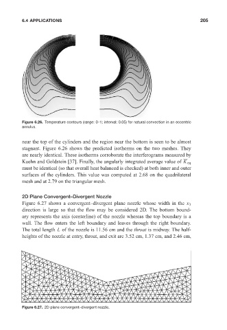
2D Plane Convergent–Divergent Nozzle
Figure 6.27 shows a convergent–divergent plane nozzle whose width in the x 3
direction is large so that the flow may be considered 2D. The bottom bound-
ary represents the axis (centerline) of the nozzle whereas the top boundary is a
wall. The flow enters the left boundary and leaves through the right boundary.
The total length L of the nozzle is 11.56 cm and the throat is midway. The half-
heights of the nozzle at entry, throat, and exit are 3.52 cm, 1.37 cm, and 2.46 cm,

Figure 6.27. 2D plane convergent–divergent nozzle.