Page 246 - Introduction to Computational Fluid Dynamics

P1: IBE
0 521 85326 5
CB908/Date
0521853265c07
7.3 1D PROBLEMS FOR IMPURE SUBSTANCES
St = 3.0 May 25, 2005 11:14 225
0.8 St = 1.0

St = 0.25
0.6

Xi(t)

0.4

0.2

DAYS
0.0
5 10 15 20
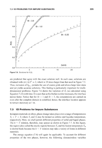
Figure 7.6. Solutions for X i (t).

are predicted that agree with the exact solution well. In each case, solutions are
2
obtained with τ/ X = 2, which is 10 times larger than that used in Figure 7.3.
Thus, inclusion of θ pc, j permits the use of coarse grids and allows large time steps
and yet yields accurate solutions. This finding is particularly important for multi-
dimensional problems. Figure 7.6 shows the variation of X i (as calculated using
Equation 7.23) with time. It is seen that as the Stefan number increases, the interface
moves faster. Notice that for St = 1 and St = 3, the computations are carried on
even after the complete domain is solidified; hence, the interface location appears
to remain stationary at 1 m.

7.3 1D Problems for Impure Substances

In impure materials or alloys, phase change takes place over a range of temperatures
T s < T < T l where T s and T l may be termed as solidus and liquidus temperature,
respectively. Here, we shall permit different properties of solid and liquid phases.
The h ∼ T relation, therefore, may appear as shown in Figure 7.7. In this figure,
the region (also called the mushy region) between T s and the fusion temperature T m
is shown blank because the h ∼ T relation may take a variety of forms in different
materials.
The energy equation (7.4) will again be applicable. To account for different
properties of the two phases, however, the following dimensionless variables