Page 290 - Introduction to Computational Fluid Dynamics

P2: IWV
P1: IWV/KCX
CB908/Date
0521853265c09
May 11, 2005
0 521 85326 5
9.5 APPLICATIONS
where δ is the change in over one iteration and R is the negative of the nodal 15:41 269
residual. Therefore, Equation 9.44 can be written as
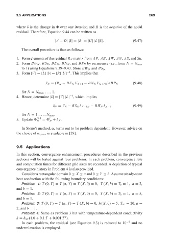
|A + D||δ|=|R|=|U||L||δ|. (9.47)
The overall procedure is thus as follows:
1. Form elements of the residual R N matrix from AP, AE, AW, AN, AS, and Su.
2. Form BW N , BS N , BE N , BN N , and BP N by recurrence (i.e., from N = N max
to 1) using Equations 9.39–9.43. Store BW N and BS N .
−1
3. Form |V |=|L||δ|=|R||U| . This implies that

V N = (R N − BE N V N+1 − BN N V N+IN )/BP N (9.48)
for N = N max ,..., 1.
−1
4. Hence, determine |δ|=|V ||L| , which implies

δ N = V N − BS N δ N−IN − BW N δ N−1 (9.49)

for N = 1,..., N max .
l
5. Update l+1 = + δ N .
N N
In Stone’s method, α s turns out to be problem dependent. However, advice on
the choice of α s,max is available in [29].

9.5 Applications

In this section, convergence enhancement procedures described in the previous
sections will be tested against four problems. In each problem, convergence rate
and computation times for different grid sizes are recorded. A depiction of typical
convergence history in Problem 4 is also provided.
Consider a rectangular domain 0 ≤ X ≤ a and 0 ≤ Y ≤ b. Assume steady-state
heat conduction with the following boundary conditions:
Problem 1: T (0, Y) = T (a, Y) = T (X, 0) = 0, T (X, b) = T b = 1, a = 2,
and b = 1.
Problem 2: T (0, Y) = T (a, Y) = T (X, 0) = 0, T (X, b) = T b = 1, a = 5,
and b = 1.
Problem 3: T (0, Y) = T (a, Y) = T (X, b) = 0, h (X, 0) = 5, T ∞ = 20, a =
2, and b = 1.
Problem 4: Same as Problem 3 but with temperature-dependent conductivity
2
k = k ref (1.0 + 0.1 T + 0.001 T ).
In each problem, the residual (see Equation 9.3) is reduced to 10 −5 and no
underrelaxation is employed.