Page 292 - Introduction to Computational Fluid Dynamics

P2: IWV
P1: IWV/KCX
0 521 85326 5
CB908/Date
0521853265c09
9.5 APPLICATIONS
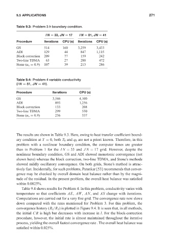
Table 9.3: Problem 3 h boundary condition. May 11, 2005 15:41 271
IN = 33, JN = 17 IN = 81, JN = 41
Procedure Iterations CPU (s) Iterations CPU (s)
GS 514 160 3,259 3,433
ADI 129 44 847 1,115
Block correction 209 77 159 242
Two-line TDMA 63 27 288 472
Stone (α s = 0.9) 107 39 213 286

Table 9.4: Problem 4 variable conductivity
(IN = 81, JN = 41).

Procedure Iterations CPU (s)
GS 3,546 4,100
ADI 893 1,256
Block correction 133 208
Two-line TDMA 299 550
Stone (α s = 0.9) 236 337

The results are shown in Table 9.3. Here, owing to heat transfer coefficient bound-
ary condition at Y = 0, both T 0 and q 0 are not a priori known. Therefore, in this
problem with a nonlinear boundary condition, the computer times are greater
than in Problem 1 for the IN = 33 and JN = 17 grid. However, despite the
nonlinear boundary condition, GS and ADI showed monotonic convergence (not
shown here) whereas the block correction, two-line TDMA, and Stone’s methods
showed mildly oscillatory convergence. On both grids, Stone’s method is attrac-
tively fast. Incidentally, for such problems, Patankar [53] recommends that conver-
gence may be checked by overall domain heat balance rather than by the magni-
tude of the residual. In the present problem, the overall heat balance was satisfied
within 0.0025%.
Table 9.4 shows results for Problem 4. In this problem, conductivity varies with
temperature so that coefficients AE, AW, AN, and AS change with iterations.
Computations are carried out for a very fine grid. The convergence rate now slows
down compared with the rates mentioned for Problem 3. For this problem, the
convergence history (R l /R 1 ) is plotted in Figure 9.4. It is seen that, in all methods,
the initial CR is high but decreases with increase in l. For the block-correction
procedure, however, the initial rate is almost maintained throughout the iterative
process, yielding the overall fastest convergence rate . The overall heat balance was
satisfied within 0.025%.