Page 100 - Introduction to Information Optics

2.4. Fourier Transform Processing KS

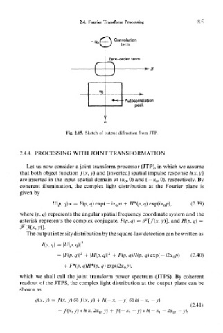
Convolution
term

Autocorrelation
peak

Fig. 2.15. Sketch of output diffraction from JTP.

2.4.4. PROCESSING WITH JOINT TRANSFORMATION

Let us now consider a joint transform processor (JTP), in which we assume
that both object function /(x, y) and (inverted) spatial impulse response /i(x. y)
are inserted in the input spatial domain at (a 0,0) and (— a 0,0), respectively. By
coherent illumination, the complex light distribution at the Fourier plane is
given by
U(p, q)* = F(p, q) exp( H*(p, q) exp(ia 0p), (2.39)

where (p, q) represents the angular spatial frequency coordinate system and the
asterisk represents the complex conjugate, F(p, q} — ^[/(x, y)], and H(p, q) —
^[_h(x, y}].
The output intensity distribution by the square-law detection can be written as

2
2
= |F(p, q)\ + \H(p, q)\ + F(p, q)H(p, q) exp(-i (2.40)
+ F*(p, q)H*(p, q) exp(i2a 0/>),
which we shall call the joint transform power spectrum (JTPS). By coherent
readout of the JTPS, the complex light distribution at the output plane can be
shown as
(x, y) - f(x, y) (g) /(x, y) + h(-x, -y) <g) h(-x, -y)
(2.4 r
+ f(x, y) * h(x, 2a 0, y) + /'(- x, - y) *h(- x, - 2a 0,