Page 196 - Introduction to Information Optics

3.2. Light Propagation in Optical Fibers 18 i

between the two curves. Note that in this case, V = \ .02 is not within the range
[1.2, 2.4]. Again, this confirms the requirement of 1.2 < V < 2.4 when Eq,
(3.36) is used.

Before the end of this section, we would like to provide percentage power
of energy inside the core, r\, under Gaussian approximation.

Pcore J T JO 2a2 w
- ° '_J1111L_L = \ -e~ ' \ (337)
' P . f
cladding J,
where w is determined by Eq. (3.36). Thus, w is in fact a function of normalized
frequency V. It can be calculated that when V= 2, about 75% light energy is
within the core. However, when V becomes smaller, the percentage of light
energy within the core also becomes smaller.

3.2.3.4. Dispersions for Single Mode Fiber
Dispersion in fiber optics is related to the bit rate or bandwidth of
fiber-optic communication systems. Due to dispersion, the narrow input pulse
will broaden after propagating in an optical fiber. As discussed in the previous
sections, different modes may have different propagating constants, /? mn. Thus,
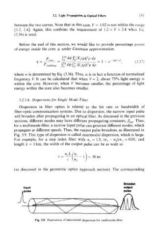
for a multimode fiber, a narrow input pulse can generate different modes, which
propagate at different speeds. Thus, the output pulse broadens, as illustrated in
Fig. 3.9. This type of dispersion is called intermodal dispersion, which is large.
For example, for a step index fiber with n l = 1.5, (n l - n 2)/n l = 0.01, and
length L = 1 km, the width of the output pulse can be as wide as

T _ _J ___L _ }
c \n~,

(as discussed in the geometric optics approach section). The corresponding

Broaden
Input output
I pulse

Fig. 3.9. Illustration of intermodal dispersion for multimode fiber.