Page 225 - Introduction to Information Optics

210 4. Switching with Optics

I 0.8

a 0.6
a

a; 0.4
a»
DC

0 1 2 3
Input Power (P/P C)

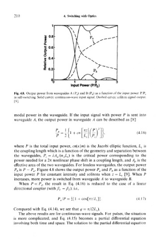
Fig. 4.8. Output power from waveguides A (P a) and B (P b) as a function of the input power P/P C
in self-switching. Solid curves: continuous-wave input signal. Dashed curves: soliton signal output.
[9].

modal power in the waveguide. If the input signal with power P is sent into
waveguide A, the output power in waveguide A can be described as [8]

nz P\ 2
(4.16)

where P is the total input power, cn(x\m) is the Jacobi elliptic function, L c is
the coupling length which is a function of the geometry and separation between
the waveguides, P c = AA e/(n 2L c) is the critical power corresponding to the
power needed for a 2n nonlinear phase shift in a coupling length, and A e is the
effective area of the two waveguides. For lossless waveguides, the output power
P h is P — P a. Figure 4.8 shows the output power P a and P b as a function of the
input power P for constant intensity and solitons when z = L c [9], When P
increases, more power is switched from waveguide A to waveguide B.
When P « P c, the result in Eq. (4.16) is reduced to the case of a linear
directional coupler (with /i, = /? 2); i.e.,

P /p _ if COS[7TZ/LJ}. (4.1?)
"«/" —2 V
Compared with Eq. (4.14), we see that g = n/(2L c).
The above results are for continuous-wave signals. For pulses, the situation
is more complicated, and Eq. (4.15) becomes a partial differential equation
involving both time and space. The solution to the partial differential equation