Page 41 - Introduction to Information Optics

26 1. Entropy Information and Optics

J
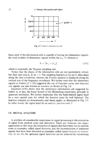
1 3AVm
AVAt =
2AVm

AVm

0 At 2At 3At 4At T
** f
Fig. 1.7. Gabor's information cell

Since each of the information cells is capable of having two elementary signals,
the total number of elementary signals within the (v m ,T) domain is

N = v mT, (1.92)
which is essentially the Nyquist sampling rate.
Notice that the shapes of the information cells are not particularly critical,
but their unit area is, AvAf = 1. The sampling function as we see it takes place
along the time coordinate, whereas the Fourier analysis is displayed along the
vertical axis of the frequency coordinate. We further note that the elementary-
signals as Gabor [1.7,1.8] suggested the use of Gaussine cosine and Gaussian
sine signals, are also known as wavelets, as shown in Fig. 1.8.
Equation (1.91) shows that the elementary information cell suggested by
Gabor is, in fact, the lower bound of the Heisenberg uncertainty principle in
quantum mechanics. We further emphasize that the band-limited signal must
be a very special type, for which the function must be well behaved. The
function contains no discontinuity and sharp angles, as illustrated in Fig. 1.9.
In other words, the signal must be an analytic function over T.

1.5. SIGNAL ANALYSIS

A problem of considerable importance in signal processing is the extraction
of signal from random noise and distortion. There are, however, two major
approaches to this issue; the extraction of signals that have been lost in random
noise as examples, called signal detection, and the reconstruction of unknown
signals that have been distorted as examples, called signal recovery or restora-
tion. As we see, the optimum signal detection can be achieved by maximizing