Page 610 - Introduction to Information Optics

594 10. Sensing with Optics

AM/W
sensing fiber
v - Av
I

Av'BriUouitt frequency shift

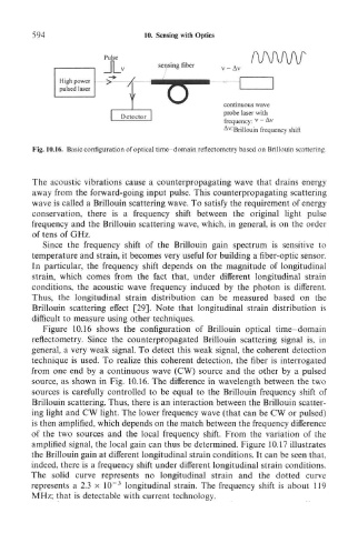
Fig. 10.16. Basic configuration of optical time-domain reflectometry based on Brillouin scattering.

The acoustic vibrations cause a counterpropagating wave that drains energy
away from the forward-going input pulse. This counterpropagating scattering
wave is called a Brillouin scattering wave. To satisfy the requirement of energy
conservation, there is a frequency shift between the original light pulse
frequency and the Brillouin scattering wave, which, in general, is on the order
of tens of GHz.
Since the frequency shift of the Brillouin gain spectrum is sensitive to
temperature and strain, it becomes very useful for building a fiber-optic sensor.
In particular, the frequency shift depends on the magnitude of longitudinal
strain, which comes from the fact that, under different longitudinal strain
conditions, the acoustic wave frequency induced by the photon is different.
Thus, the longitudinal strain distribution can be measured based on the
Brillouin scattering effect [29]. Note that longitudinal strain distribution is
difficult to measure using other techniques.
Figure 10.16 shows the configuration of Brillouin optical time-domain
reflectometry. Since the counterpropagated Brillouin scattering signal is, in
general, a very weak signal. To detect this weak signal, the coherent detection
technique is used. To realize this coherent detection, the fiber is interrogated
from one end by a continuous wave (CW) source and the other by a pulsed
source, as shown in Fig. 10.16. The difference in wavelength between the two
sources is carefully controlled to be equal to the Brillouin frequency shift of
Brillouin scattering. Thus, there is an interaction between the Brillouin scatter-
ing light and CW light. The lower frequency wave (that can be CW or pulsed)
is then amplified, which depends on the match between the frequency difference
of the two sources and the local frequency shift. From the variation of the
amplified signal, the local gain can thus be determined. Figure 10.17 illustrates
the Brillouin gain at different longitudinal strain conditions. It can be seen that,
indeed, there is a frequency shift under different longitudinal strain conditions.
The solid curve represents no longitudinal strain and the dotted curve
3
represents a 2.3 x 10 ~ longitudinal strain. The frequency shift is about 119
MHz; that is detectable with current technology.