Page 326 - Introduction to chemical reaction engineering and kinetics

12.3 Design Equations for a Batch Reactor 307
-
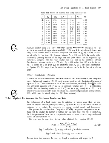
Table 12.2 Results for Example 12-5 using trapezoidal rule
j
t/h
G
T/K
r 0.00 300.0 kAh-’ 3.00 0.00
fA
0.334
2 0.10 303.4 0.484 2.29 2.65 0.26
3 0.20 306.8 0.696 1.79 2.04 0.47
4 0.30 310.2 0.994 1.44 1.62 0.63
5 0.40 313.5 1.408 1.18 1.31 0.76
6 0.50 316.9 1.979 1.01 1.10 0.87
7 0.60 320.3 2.762 0.91 0.96 0.97
8 0.70 323.7 3.828 0.87 0.89 1.06
9 0.80 327.1 5.269 0.95 0.91 1.15
10 0.90 330.5 7.206 10.53 5.96 1.26
1.39
1.17
0 Alternate solution using E-Z Solve sofnuare: (see file exl2-5.msp). The results for t us-
11
333.5
0.99
9.500
1.80
-
*
V
7O-v
ing the trapezoidal rule approximation (Table 12.2) may differ significantly from those
using a more accurate form of numerical integration. For values of fA up to 0.90, the val-
ues oft differ by less than 1%. However, between fA = 0.90 and 0.99, the results differ
considerably, primarily because of the large step size (0.09) chosen for the trapezoidal ap-
proximation, compared with the much smaller step size used in the simulation software.
The simulation software predicts t = 1.52 h for fA = 0.99, rather than 1.80 h as in the ta-
ble. The results for T (at given fA) are unaffected, since fA and T are related algebraically
by Equation (C). The output from the simulation software can be in the form of a table or
graph.
12.3.3.2 Nonadiabatic Operation
as dependent variables and t
If the batch reactor operation is both nonadiabatic and nonisothermal, the complete
energy balance of equation 12.3-16 must be used together with the material balance of
equation 2.2-4. These constitute a set of two simultaneous, nonlinear, first-order ordi-
nary differential equations with T and fA = fAO (usually 0) att = 0.
as independent
0 These two equations usually must be solved by a numerical procedure. (See problem
variable. The two boundary conditions are T = T, and fA
V
12-9, which may be solved using the E-Z Solve software.)
7O-v
12.3.4 Optimal Performance for Maximum Production Rate

The performance of a batch reactor may be optimized in various ways. Here, we con-
sider the case of choosing the cycle time, t,, equation 12.3-5, to maximize the rate of
production of a product. For simplicity, we assume constant density and temperature.
The greater the reaction time t (equation 12.3-21), the greater the production per
batch, but the smaller the number of batches per unit time. Since the rate of production,
Pr, is the product of these two, a compromise must be made between large and small
values oft to maximize Pr.
This may also be seen from limiting values obtained from equation 12.3-22:

Pr(C) = kcAov(fA2 - fA1) (12.3-22)
t + td
hy Pr = 0, since fA2 - fAl 4 0 and td is a finite constant
lim Pr = 0, since fA2 - fA1 * a constant
t-+m
Between these two extremes, Pr must go through a maximum with respect to t .