Page 85 - Low Temperature Energy Systems with Applications of Renewable Energy

74 Low-Temperature Energy Systems with Applications of Renewable Energy

Equation (2.13), and the temperature of the working fluid being fed into the heating
system from Eq. (2.15), we obtain the curves shown in Fig. 2.18.
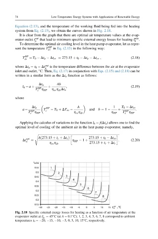
It is clear from the graph that there are optimal air temperature values at the evap-
orator outlet t out that lead to minimum specific external energy losses for heating l min .
a h
To determine the optimal air cooling level in the heat pump evaporator, let us repre-
sent the temperature T HP in Eq. (2.15) in the following way:
ev
HP
T ¼ T 0 Dt a Dt ev ¼ 273:15 þ t 0 Dt a Dt ev ; (2.18)
ev
where Dt a ¼ t 0 Dt out is the temperature difference between the air at the evaporator
a

inlet and outlet, C. Then, Eq. (2.17) in conjunction with Eqs. (2.15) and (2.18) can be
written in a similar form as the Dt a function as follows:
Dt a Ab
l h ¼ a þ þ ; (2.19)
T HP h
ev dr
c HP h h Dt a
where

Dt a HP A 1 T 0 Dt ev
a ¼ HP T c T 0 þ DT ev and b ¼ 1 þ HP :
T h h h h T h
c HP ev dr HP c HP
Applying the calculus of variations to the function l h ¼ f(Dt a ) allows one to find the
optimal level of cooling of the ambient air in the heat pump evaporator, namely,

s ffiffiffiffiffiffiffiffiffiffiffiffiffiffiffiffiffiffiffiffiffiffiffiffiffiffiffiffiffiffiffiffiffiffiffiffiffiffiffiffiffiffiffiffiffiffiffiffiffiffiffiffiffiffiffiffiffiffiffiffiffiffiffiffiffiffiffiffiffiffiffiffiffiffiffiffiffiffiffiffiffiffiffiffiffiffiffiffiffiffiffiffiffiffiffiffiffiffiffiffiffiffiffiffiffiffiffi
273:15 þ t 0 Dt ev
Að273:15 þ t c þ Dt c Þ
Dt opt ¼ h HP 1 þ : (2.20)
a
h h 273:15 þ t c þ Dt c
ev dr

Fig. 2.18 Specific external energy losses for heating as a function of air temperature at the

evaporator outlet at t c ¼ 45 C (at A ¼ 0.1 C); 1, 2, 3, 4, 5, 6, 7, 8 correspond to ambient
hc

temperatures t 0 ¼ 20, 15, 10, 5, 0, 5, 10, 15 C, respectively.