Page 217 - MATLAB an introduction with applications

202 ——— MATLAB: An Introduction with Applications

 A 11 A 12 A 13 " A 1k " A 1j " A 1n  
b
1
  
b
 0 A 22 A 23 " A 2k " A 2 j " A 2n  
2
 0 0 A 33 " A 3k " A 3 j " A  
b
3n
3
  
#
 # # # # # # # # #  
 0 0 0 " A " A " A   pivot row
b
k ←
 kk kj kn  
#
#  # # # # # # # #  
 0 0 0 " A " A " A   ...(4.2)
b
i ←
 ik ij in    row being transformed
#  # # # # # # # #   # 
   
b
  0 0 0 " A nk " A nj " A nn    

n
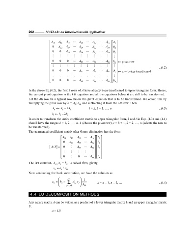
In the above Eq.(4.2), the first k rows of A have already been transformed to upper triangular form. Hence,
the current pivot equation is the kth equation and all the equations below it are still to be transformed.
Let the ith row be a typical row below the pivot equation that is to be transformed. We obtain this by
multiplying the pivot row by λ = A /A and subtracting it from the i-th row. Then
kk
ik
A ← A − λ A j = k, k + 1, …, n ...(4.3)
ij ij kj
b ← b − λ b
i i k
In order to transform the entire coefficient matrix to upper triangular form, k and i in Eqs. (4.3) and (4.4)
should have the ranges k = 1, 2, …, n–1 (choose the pivot row), i = k + 1, k + 2, …, n (selects the row to
be transformed).
The augmented coefficient matrix after Gauss elimination has the form
b
 A 11 A 12 A 13 " A 1n   
1
 0 A A " A   
b
 22 23 2n   
2
b
[ / ] =  0 0 A 33 " A   
Ab
3
3n
   
#
 # # # # #   
  0 0 0 " A nn   
  
b
n
The last equation, A x = b , is solved first, giving
n
n
nn
x = b n / A nn
n
Now conducting the back substitution, we have the solution as
 n  1
k ∑
x =  b − A x j  k = n – 1, n – 2, … ...(4.4)
k
kj
 jk 1  A kk
=+
4.4 LU DECOMPOSITION METHODS
Any square matrix A can be written as a product of a lower triangular matrix L and an upper triangular matrix
U.
A = LU