Page 222 - MATLAB an introduction with applications

Numerical Methods ——— 207

r
provided ([I] – [B]) is non-singular. Here we see that as r → ∞ the limit of the sum exists if [B] → 0, in this
case s → s = ([I] – [B]) .
–1

r
r
r
Hence in Eq.(4.13) x will converge to the vector {x} provided [B] → 0 as r → ∞. Then the vector {x}
can be written as
–1
{x} = ([I] – [B] {v})
This means that ([I] – [B]) {x} = (v) and hence {x} = [B]{x} + {v}. This is just the equation (4.12).
4.9 THE HOUSEHOLDER FACTORIZATION

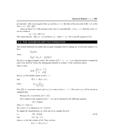
This method transforms the matrix into an upper triangular form by making use of reflection matrices; we
have
[P ] [A]
T
H
where
T
T
T
[P ] = [P ] … [P ] [P ] T
H
1
2
n–1
T
The [S ] is an upper triangular matrix. The matrices [P ] , i = 1, ..., n – 1 are reflection matrices computed in
H
i
T
such a way that [P ] reduce the subdiagonal elements in column i of the coefficient matrix.
i
Then we have
 [I ] 0 
[]PT =  i− 1 
i
P
 0 [ ]
i 
here [I ] is the identity matrix of size i – 1
i–1

T
and []P = 1 – θ{w} {w} ;
i
2
where θ=
T
{} { }
w
w
i
i

Here []P is a symmetric matrix and {w } is a vector of size n – i + 1. The vector {w } will be chosen as
i
i
i
explained later.

T
P
Because [] is symmetric, [P ] = [P ].
i
i
i
Now solution of the equation [A]{x} = {b} can be obtained by the following equation
[A] = [P ][S ]
H
H
where {v} = [S ] {x}.
H
The vector {v} is obtained as {v}= [P ] {b}.
T
H
To explain the transformation, as a first step let us compute the [P ],
1

A
i.e., [] = [P ][A] ...(4.14)
1
and [A] = [a ; A ]
1
1
where a is the first column of [A]. Then, we have
1
[P ] = I – θ{w }{w } T
1
1
1